Multidimensional models

Fitting is not limited to 1D models. The following example demonstrates how to fit a 2D Gaussian peak to a 2D DataArray.

import numpy as np
import xarray as xr
import matplotlib.pyplot as plt
import lmfit
import xarray_lmfit

# Generate synthetic 2D data
x = np.linspace(-10, 10, 50)
y = np.linspace(-10, 10, 50)
x_arr = xr.DataArray(x, dims=("x",), coords={"x": x})
y_arr = xr.DataArray(y, dims=("y",), coords={"y": y})
z_arr = lmfit.lineshapes.gaussian2d(
    x_arr,
    y_arr,
    amplitude=4.0,
    centerx=0.0,
    centery=0.0,
    sigmax=1.0,
    sigmay=2.0,
).rename("z")

# Add some noise with fixed seed for reproducibility
rng = np.random.default_rng(5)
z_arr = z_arr.copy(data=rng.normal(z_arr, 0.01))

Fitting a 2D model is as simple as providing multiple coordinate names for different independent variables:

model = lmfit.models.Gaussian2dModel()

result_ds = z_arr.xlm.modelfit(
    ("x", "y"),
    model=model,
    params=model.make_params(
        amplitude=2.0, centerx=0.0, centery=0.0, sigmax=1.0, sigmay=2.0
    ),
)
result_ds

<xarray.Dataset> Size: 43kB
Dimensions:                (param: 8, cov_i: 8, cov_j: 8, fit_stat: 9, x: 50,
                            y: 50)
Coordinates:
  * x                      (x) float64 400B -10.0 -9.592 -9.184 ... 9.592 10.0
  * y                      (y) float64 400B -10.0 -9.592 -9.184 ... 9.592 10.0
  * param                  (param) <U9 288B 'amplitude' 'centerx' ... 'height'
  * fit_stat               (fit_stat) <U8 288B 'nfev' 'nvarys' ... 'rsquared'
  * cov_i                  (cov_i) <U9 288B 'amplitude' 'centerx' ... 'height'
  * cov_j                  (cov_j) <U9 288B 'amplitude' 'centerx' ... 'height'
Data variables:
    modelfit_results       object 8B <lmfit.model.ModelResult object at 0x73d...
    modelfit_coefficients  (param) float64 64B 4.065 -0.006079 ... 4.778 0.3158
    modelfit_stderr        (param) float64 64B 0.02927 0.00727 ... 0.002274
    modelfit_covariance    (cov_i, cov_j) float64 512B 0.0008566 ... nan
    modelfit_stats         (fit_stat) float64 72B 25.0 5.0 ... -2.3e+04 0.9355
    modelfit_data          (x, y) float64 20kB -0.008019 -0.01324 ... 0.001742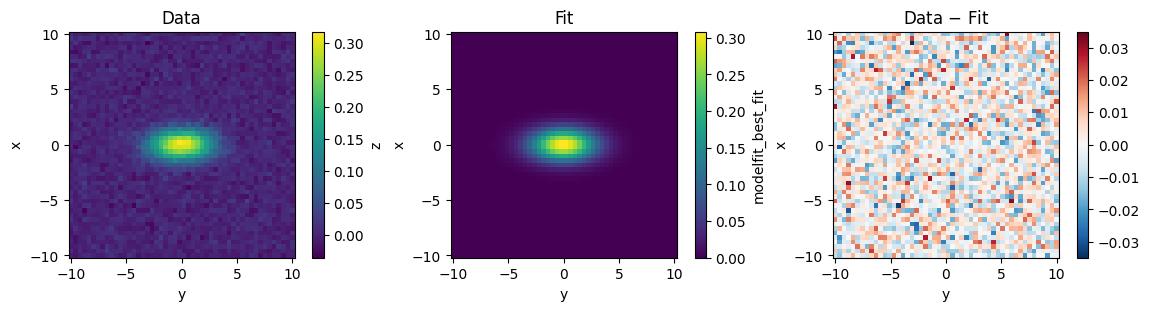
    modelfit_best_fit      (x, y) float64 20kB 9.16e-28 2.416e-27 ... 7.671e-28

xarray.Dataset

• Dimensions:
  • param: 8
  • cov_i: 8
  • cov_j: 8
  • fit_stat: 9
  • x: 50
  • y: 50
• Coordinates: (6)
  • x
    (x)
    float64
    -10.0 -9.592 -9.184 ... 9.592 10.0

    array([-10.      ,  -9.591837,  -9.183673,  -8.77551 ,  -8.367347,  -7.959184,
            -7.55102 ,  -7.142857,  -6.734694,  -6.326531,  -5.918367,  -5.510204,
            -5.102041,  -4.693878,  -4.285714,  -3.877551,  -3.469388,  -3.061224,
            -2.653061,  -2.244898,  -1.836735,  -1.428571,  -1.020408,  -0.612245,
            -0.204082,   0.204082,   0.612245,   1.020408,   1.428571,   1.836735,
             2.244898,   2.653061,   3.061224,   3.469388,   3.877551,   4.285714,
             4.693878,   5.102041,   5.510204,   5.918367,   6.326531,   6.734694,
             7.142857,   7.55102 ,   7.959184,   8.367347,   8.77551 ,   9.183673,
             9.591837,  10.      ])

  • y
    (y)
    float64
    -10.0 -9.592 -9.184 ... 9.592 10.0

    array([-10.      ,  -9.591837,  -9.183673,  -8.77551 ,  -8.367347,  -7.959184,
            -7.55102 ,  -7.142857,  -6.734694,  -6.326531,  -5.918367,  -5.510204,
            -5.102041,  -4.693878,  -4.285714,  -3.877551,  -3.469388,  -3.061224,
            -2.653061,  -2.244898,  -1.836735,  -1.428571,  -1.020408,  -0.612245,
            -0.204082,   0.204082,   0.612245,   1.020408,   1.428571,   1.836735,
             2.244898,   2.653061,   3.061224,   3.469388,   3.877551,   4.285714,
             4.693878,   5.102041,   5.510204,   5.918367,   6.326531,   6.734694,
             7.142857,   7.55102 ,   7.959184,   8.367347,   8.77551 ,   9.183673,
             9.591837,  10.      ])

  • param
    (param)
    <U9
    'amplitude' 'centerx' ... 'height'

    array(['amplitude', 'centerx', 'centery', 'sigmax', 'sigmay', 'fwhmx', 'fwhmy',
           'height'], dtype='<U9')

  • fit_stat
    (fit_stat)
    <U8
    'nfev' 'nvarys' ... 'rsquared'

    array(['nfev', 'nvarys', 'ndata', 'nfree', 'chisqr', 'redchi', 'aic', 'bic',
           'rsquared'], dtype='<U8')

  • cov_i
    (cov_i)
    <U9
    'amplitude' 'centerx' ... 'height'

    array(['amplitude', 'centerx', 'centery', 'sigmax', 'sigmay', 'fwhmx', 'fwhmy',
           'height'], dtype='<U9')

  • cov_j
    (cov_j)
    <U9
    'amplitude' 'centerx' ... 'height'

    array(['amplitude', 'centerx', 'centery', 'sigmax', 'sigmay', 'fwhmx', 'fwhmy',
           'height'], dtype='<U9')

• Data variables: (7)
  • modelfit_results
    ()
    object
    <lmfit.model.ModelResult object ...

    array(<lmfit.model.ModelResult object at 0x73d3a910c8c0>, dtype=object)

  • modelfit_coefficients
    (param)
    float64
    4.065 -0.006079 ... 4.778 0.3158

    array([ 4.06470897, -0.00607853, -0.01196016,  1.00965373,  2.0290147 ,
            2.37755281,  4.77796439,  0.31578524])

  • modelfit_stderr
    (param)
    float64
    0.02927 0.00727 ... 0.0344 0.002274

    array([0.0292684 , 0.00727004, 0.01461018, 0.00727014, 0.01461034,
           0.01711986, 0.03440473, 0.00227385])

  • modelfit_covariance
    (cov_i, cov_j)
    float64
    0.0008566 1.093e-13 ... nan nan

    array([[ 8.56639517e-04,  1.09327264e-13, -6.61914892e-14,
             1.06393294e-04,  2.13811737e-04,             nan,
                        nan,             nan],
           [ 1.09327264e-13,  5.28534831e-05,  7.66118832e-15,
            -1.59433972e-12,  2.28249775e-14,             nan,
                        nan,             nan],
           [-6.61914892e-14,  7.66118832e-15,  2.13457272e-04,
            -1.08962652e-15, -6.44217209e-12,             nan,
                        nan,             nan],
           [ 1.06393294e-04, -1.59433972e-12, -1.08962652e-15,
             5.28548986e-05,  3.93867830e-17,             nan,
                        nan,             nan],
           [ 2.13811737e-04,  2.28249775e-14, -6.44217209e-12,
             3.93867830e-17,  2.13462166e-04,             nan,
                        nan,             nan],
           [            nan,             nan,             nan,
                        nan,             nan,             nan,
                        nan,             nan],
           [            nan,             nan,             nan,
                        nan,             nan,             nan,
                        nan,             nan],
           [            nan,             nan,             nan,
                        nan,             nan,             nan,
                        nan,             nan]])

  • modelfit_stats
    (fit_stat)
    float64
    25.0 5.0 ... -2.3e+04 0.9355

    array([ 2.50000000e+01,  5.00000000e+00,  2.50000000e+03,  2.49500000e+03,
            2.49167241e-01,  9.98666297e-05, -2.30241924e+04, -2.29950722e+04,
            9.35471566e-01])

  • modelfit_data
    (x, y)
    float64
    -0.008019 -0.01324 ... 0.001742

    array([[-0.00801931, -0.01324359, -0.00248362, ..., -0.0198843 ,
            -0.00233423, -0.0025579 ],
           [ 0.00962001, -0.01181447,  0.00738042, ...,  0.00265091,
            -0.00464245, -0.00478638],
           [-0.00721316, -0.0051976 ,  0.00160227, ...,  0.01092893,
            -0.01058737,  0.01375824],
           ...,
           [-0.00242389,  0.01999988, -0.00546568, ..., -0.01504261,
            -0.01028359, -0.00643577],
           [ 0.02279287,  0.00285862,  0.01808877, ..., -0.00117906,
             0.00948935, -0.00093704],
           [ 0.00994932, -0.00549919, -0.00023564, ...,  0.00385409,
             0.0103395 ,  0.00174165]], shape=(50, 50))

  • modelfit_best_fit
    (x, y)
    float64
    9.16e-28 2.416e-27 ... 7.671e-28

    array([[9.16001368e-28, 2.41639519e-27, 6.12160570e-27, ...,
            5.80352082e-27, 2.28541046e-27, 8.64295841e-28],
           [4.61579279e-26, 1.21763786e-25, 3.08471847e-25, ...,
            2.92443336e-25, 1.15163377e-25, 4.35524514e-26],
           [1.97524598e-24, 5.21066349e-24, 1.32005011e-23, ...,
            1.25145896e-23, 4.92821079e-24, 1.86374928e-24],
           ...,
           [1.77033931e-24, 4.67012337e-24, 1.18311168e-23, ...,
            1.12163600e-23, 4.41697154e-24, 1.67040897e-24],
           [4.11687466e-26, 1.08602416e-25, 2.75129320e-25, ...,
            2.60833320e-25, 1.02715441e-25, 3.88448945e-26],
           [8.13024209e-28, 2.14474329e-27, 5.43341288e-27, ...,
            5.15108721e-27, 2.02848390e-27, 7.67131434e-28]], shape=(50, 50))

• Indexes: (6)
  • x
    PandasIndex

    PandasIndex(Index([              -10.0,  -9.591836734693878,  -9.183673469387756,
            -8.775510204081632,   -8.36734693877551,  -7.959183673469388,
            -7.551020408163265,  -7.142857142857142,   -6.73469387755102,
            -6.326530612244898,  -5.918367346938775, -5.5102040816326525,
           -5.1020408163265305, -4.6938775510204085,  -4.285714285714286,
           -3.8775510204081627, -3.4693877551020407, -3.0612244897959187,
           -2.6530612244897958,  -2.244897959183673, -1.8367346938775508,
           -1.4285714285714288,  -1.020408163265305,  -0.612244897959183,
            -0.204081632653061,   0.204081632653061,   0.612244897959183,
            1.0204081632653068,  1.4285714285714288,  1.8367346938775508,
            2.2448979591836746,  2.6530612244897966,  3.0612244897959187,
            3.4693877551020407,  3.8775510204081627,  4.2857142857142865,
            4.6938775510204085,  5.1020408163265305,   5.510204081632654,
             5.918367346938776,   6.326530612244898,    6.73469387755102,
             7.142857142857142,   7.551020408163264,    7.95918367346939,
             8.367346938775512,   8.775510204081634,   9.183673469387756,
             9.591836734693878,                10.0],
          dtype='float64', name='x'))

  • y
    PandasIndex

    PandasIndex(Index([              -10.0,  -9.591836734693878,  -9.183673469387756,
            -8.775510204081632,   -8.36734693877551,  -7.959183673469388,
            -7.551020408163265,  -7.142857142857142,   -6.73469387755102,
            -6.326530612244898,  -5.918367346938775, -5.5102040816326525,
           -5.1020408163265305, -4.6938775510204085,  -4.285714285714286,
           -3.8775510204081627, -3.4693877551020407, -3.0612244897959187,
           -2.6530612244897958,  -2.244897959183673, -1.8367346938775508,
           -1.4285714285714288,  -1.020408163265305,  -0.612244897959183,
            -0.204081632653061,   0.204081632653061,   0.612244897959183,
            1.0204081632653068,  1.4285714285714288,  1.8367346938775508,
            2.2448979591836746,  2.6530612244897966,  3.0612244897959187,
            3.4693877551020407,  3.8775510204081627,  4.2857142857142865,
            4.6938775510204085,  5.1020408163265305,   5.510204081632654,
             5.918367346938776,   6.326530612244898,    6.73469387755102,
             7.142857142857142,   7.551020408163264,    7.95918367346939,
             8.367346938775512,   8.775510204081634,   9.183673469387756,
             9.591836734693878,                10.0],
          dtype='float64', name='y'))

  • param
    PandasIndex

    PandasIndex(Index(['amplitude', 'centerx', 'centery', 'sigmax', 'sigmay', 'fwhmx', 'fwhmy',
           'height'],
          dtype='object', name='param'))

  • fit_stat
    PandasIndex

    PandasIndex(Index(['nfev', 'nvarys', 'ndata', 'nfree', 'chisqr', 'redchi', 'aic', 'bic',
           'rsquared'],
          dtype='object', name='fit_stat'))

  • cov_i
    PandasIndex

    PandasIndex(Index(['amplitude', 'centerx', 'centery', 'sigmax', 'sigmay', 'fwhmx', 'fwhmy',
           'height'],
          dtype='object', name='cov_i'))

  • cov_j
    PandasIndex

    PandasIndex(Index(['amplitude', 'centerx', 'centery', 'sigmax', 'sigmay', 'fwhmx', 'fwhmy',
           'height'],
          dtype='object', name='cov_j'))

• Attributes: (0)

Let’s take a look at the best fit and residuals:

fig, axs = plt.subplots(1, 3, figsize=(12, 3), layout="compressed")

z_arr.plot(ax=axs[0], center=False)
axs[0].set_title("Data")

result_ds.modelfit_best_fit.plot(ax=axs[1])
axs[1].set_title("Fit")

(z_arr - result_ds.modelfit_best_fit).plot(ax=axs[2])
axs[2].set_title("Data $-$ Fit")

for ax in axs:
    ax.set_aspect("equal")