Fitting across multiple dimensions#
Suppose you have to fit a single model to multiple data points across some dimension, or even multiple dimensions. The accessor can handle this with ease.
To demonstrate, let’s extend our previous example of fitting a 1D Gaussian peak on a linear background to 2D, where each row contains a Gaussian peak with a different center.
import numpy as np
import xarray as xr
import matplotlib.pyplot as plt
import lmfit
import xarray_lmfit
# Define coordinates
x = np.linspace(-5.0, 5.0, 100)
y = np.arange(3)

# Center of the peaks along y
center = np.array([-2.0, 0.0, 2.0])[:, np.newaxis]

# Gaussian peak on a linear background
z = -0.1 * x + 2 + 3 * np.exp(-((x - center) ** 2) / (2 * 1**2))

# Add some noise with fixed seed for reproducibility
rng = np.random.default_rng(5)
zerr = np.full_like(z, 0.1)
z = rng.normal(z, zerr)

# Construct DataArray
darr = xr.DataArray(z, dims=["y", "x"], coords={"y": y, "x": x})
darr.plot()
<matplotlib.collections.QuadMesh at 0x702b48685c10>

xarray.DataArray.xlm.modelfit() will automatically broadcast the model parameters across the non-fitting dimensions, allowing you to fit all rows in one go.
model = lmfit.models.GaussianModel() + lmfit.models.LinearModel()

params = {"center": 0.0, "slope": -0.1}

result_ds = darr.xlm.modelfit(coords="x", model=model, params=params)
result_ds
<xarray.Dataset> Size: 8kB
Dimensions:                (y: 3, param: 5, cov_i: 5, cov_j: 5, fit_stat: 9,
                            x: 100)
Coordinates:
  * y                      (y) int64 24B 0 1 2
  * x                      (x) float64 800B -5.0 -4.899 -4.798 ... 4.899 5.0
  * param                  (param) <U9 180B 'amplitude' 'center' ... 'intercept'
  * fit_stat               (fit_stat) <U8 288B 'nfev' 'nvarys' ... 'rsquared'
  * cov_i                  (cov_i) <U9 180B 'amplitude' 'center' ... 'intercept'
  * cov_j                  (cov_j) <U9 180B 'amplitude' 'center' ... 'intercept'
Data variables:
    modelfit_results       (y) object 24B <lmfit.model.ModelResult object at ...
    modelfit_coefficients  (y, param) float64 120B 7.324 -2.0 ... -0.1044 1.993
    modelfit_stderr        (y, param) float64 120B 0.1349 0.011 ... 0.01735
    modelfit_covariance    (y, cov_i, cov_j) float64 600B 0.01819 ... 0.0003009
    modelfit_stats         (y, fit_stat) float64 216B 51.0 5.0 ... -450.2 0.9895
    modelfit_data          (y, x) float64 2kB 2.453 2.402 2.515 ... 1.404 1.64
modelfit_best_fit (y, x) float64 2kB 2.553 2.553 2.557 ... 1.526 1.504- y: 3
- param: 5
- cov_i: 5
- cov_j: 5
- fit_stat: 9
- x: 100
- y(y)int640 1 2
array([0, 1, 2])
- x(x)float64-5.0 -4.899 -4.798 ... 4.899 5.0
array([-5. , -4.89899 , -4.79798 , -4.69697 , -4.59596 , -4.494949, -4.393939, -4.292929, -4.191919, -4.090909, -3.989899, -3.888889, -3.787879, -3.686869, -3.585859, -3.484848, -3.383838, -3.282828, -3.181818, -3.080808, -2.979798, -2.878788, -2.777778, -2.676768, -2.575758, -2.474747, -2.373737, -2.272727, -2.171717, -2.070707, -1.969697, -1.868687, -1.767677, -1.666667, -1.565657, -1.464646, -1.363636, -1.262626, -1.161616, -1.060606, -0.959596, -0.858586, -0.757576, -0.656566, -0.555556, -0.454545, -0.353535, -0.252525, -0.151515, -0.050505, 0.050505, 0.151515, 0.252525, 0.353535, 0.454545, 0.555556, 0.656566, 0.757576, 0.858586, 0.959596, 1.060606, 1.161616, 1.262626, 1.363636, 1.464646, 1.565657, 1.666667, 1.767677, 1.868687, 1.969697, 2.070707, 2.171717, 2.272727, 2.373737, 2.474747, 2.575758, 2.676768, 2.777778, 2.878788, 2.979798, 3.080808, 3.181818, 3.282828, 3.383838, 3.484848, 3.585859, 3.686869, 3.787879, 3.888889, 3.989899, 4.090909, 4.191919, 4.292929, 4.393939, 4.494949, 4.59596 , 4.69697 , 4.79798 , 4.89899 , 5. ]) - param(param)<U9'amplitude' ... 'intercept'
array(['amplitude', 'center', 'sigma', 'slope', 'intercept'], dtype='<U9')
- fit_stat(fit_stat)<U8'nfev' 'nvarys' ... 'rsquared'
array(['nfev', 'nvarys', 'ndata', 'nfree', 'chisqr', 'redchi', 'aic', 'bic', 'rsquared'], dtype='<U8') - cov_i(cov_i)<U9'amplitude' ... 'intercept'
array(['amplitude', 'center', 'sigma', 'slope', 'intercept'], dtype='<U9')
- cov_j(cov_j)<U9'amplitude' ... 'intercept'
array(['amplitude', 'center', 'sigma', 'slope', 'intercept'], dtype='<U9')
- modelfit_results(y)object<lmfit.model.ModelResult object ...
array([<lmfit.model.ModelResult object at 0x702b483b7440>, <lmfit.model.ModelResult object at 0x702b483b6f60>, <lmfit.model.ModelResult object at 0x702b483ded80>], dtype=object) - modelfit_coefficients(y, param)float647.324 -2.0 0.9919 ... -0.1044 1.993
array([[ 7.3244805 , -1.99999202, 0.99188968, -0.10520867, 1.99685622], [ 7.51733234, -0.02305536, 1.0003855 , -0.09703458, 2.00966728], [ 7.59666754, 1.99366668, 0.99723651, -0.10435843, 1.99329883]]) - modelfit_stderr(y, param)float640.1349 0.011 ... 0.004993 0.01735
array([[0.13487976, 0.0109997 , 0.01456656, 0.00460003, 0.01594714], [0.10826444, 0.01195036, 0.0134014 , 0.00363877, 0.01476934], [0.14709449, 0.01159003, 0.01536977, 0.00499329, 0.01734786]]) - modelfit_covariance(y, cov_i, cov_j)float640.01819 -0.0004108 ... 0.0003009
array([[[ 1.81925505e-02, -4.10783969e-04, 1.61528942e-03, 4.48816520e-04, -1.78536072e-03], [-4.10783969e-04, 1.20993414e-04, -3.61614978e-05, -1.94839515e-05, 4.00287792e-05], [ 1.61528942e-03, -3.61614978e-05, 2.12184585e-04, 3.94801678e-05, -1.57976969e-04], [ 4.48816520e-04, -1.94839515e-05, 3.94801678e-05, 2.11602886e-05, -4.40243889e-05], [-1.78536072e-03, 4.00287792e-05, -1.57976969e-04, -4.40243889e-05, 2.54311269e-04]], [[ 1.17211884e-02, -3.23794800e-06, 1.03989191e-03, 3.42954464e-06, -1.16038807e-03], [-3.23794800e-06, 1.42811206e-04, -2.87229808e-07, -1.25020965e-05, 3.20525581e-07], [ 1.03989191e-03, -2.87229808e-07, 1.79597412e-04, 3.04209903e-07, -1.02947687e-04], [ 3.42954464e-06, -1.25020965e-05, 3.04209903e-07, 1.32406704e-05, -3.39519610e-07], [-1.16038807e-03, 3.20525581e-07, -1.02947687e-04, -3.39519610e-07, 2.18133452e-04]], [[ 2.16367879e-02, 4.77026736e-04, 1.86127523e-03, -5.32371055e-04, -2.12282188e-03], [ 4.77026736e-04, 1.34328709e-04, 4.06750352e-05, -2.24786041e-05, -4.64667181e-05], [ 1.86127523e-03, 4.06750352e-05, 2.36229982e-04, -4.53617031e-05, -1.81975941e-04], [-5.32371055e-04, -2.24786041e-05, -4.53617031e-05, 2.49329517e-05, 5.22061279e-05], [-2.12282188e-03, -4.64667181e-05, -1.81975941e-04, 5.22061279e-05, 3.00948191e-04]]]) - modelfit_stats(y, fit_stat)float6451.0 5.0 100.0 ... -450.2 0.9895
array([[ 5.10000000e+01, 5.00000000e+00, 1.00000000e+02, 9.50000000e+01, 7.51416422e-01, 7.90964655e-03, -4.79096548e+02, -4.66070697e+02, 9.94600761e-01], [ 3.10000000e+01, 5.00000000e+00, 1.00000000e+02, 9.50000000e+01, 9.80931827e-01, 1.03255982e-02, -4.52442250e+02, -4.39416399e+02, 9.91217434e-01], [ 5.80000000e+01, 5.00000000e+00, 1.00000000e+02, 9.50000000e+01, 8.80348758e-01, 9.26682904e-03, -4.63260732e+02, -4.50234881e+02, 9.89533284e-01]]) - modelfit_data(y, x)float642.453 2.402 2.515 ... 1.404 1.64
array([[2.45313385, 2.40235674, 2.51482263, 2.59074915, 2.6764208 , 2.59394952, 2.55499778, 2.56731807, 2.76560738, 2.90968187, 2.84053704, 2.76947573, 2.88970859, 3.25183004, 3.23198866, 3.17150326, 3.48156317, 3.52952886, 3.74747336, 3.93214775, 4.08299485, 4.38225482, 4.48844307, 4.59470196, 4.84031769, 5.0107361 , 4.87070097, 5.09207864, 5.07519126, 5.18226532, 5.06665073, 5.1631842 , 5.09310067, 4.9741113 , 4.78172815, 4.70632343, 4.47734082, 4.2766245 , 4.24965452, 3.9248589 , 3.95910191, 3.7214431 , 3.26250461, 3.30964501, 3.00234976, 2.95758539, 2.81323142, 2.47807647, 2.53524934, 2.42805834, 2.45768018, 2.16314796, 2.28587715, 2.04281712, 2.06893741, 1.97493843, 2.16724827, 2.04803446, 2.20774591, 2.005823 , 2.00617416, 1.98816284, 1.82771981, 1.8671122 , 1.99599647, 1.8089832 , 1.85582487, 1.82359101, 1.87574004, 1.76767498, 1.77844967, 1.80756538, 1.7833553 , 1.67633946, 1.84223817, 1.61266135, 1.61226509, 1.59400618, 1.80883879, 1.66597173, 1.59482299, 1.56822047, 1.7138329 , 1.55613362, 1.52430821, 1.70281395, 1.51164264, 1.58896847, 1.61043505, 1.55647661, 1.58549972, 1.71468544, 1.51901766, 1.43467535, 1.36683048, 1.51992743, 1.49507733, 1.54671111, 1.46367655, 1.45213615], ... [2.44598688, 2.27945239, 2.42172801, 2.46969848, 2.57847903, 2.34804814, 2.50606228, 2.50882285, 2.3492531 , 2.39033196, 2.57593497, 2.56093745, 2.46434024, 2.40188179, 2.47241732, 2.334418 , 2.32887606, 2.24224943, 2.31874259, 2.29988659, 2.57535533, 2.26861482, 2.40489271, 2.39977991, 2.23901312, 2.36454908, 2.01990284, 2.23709116, 2.30339681, 1.96804075, 2.08218813, 2.29416313, 2.15354763, 2.06045838, 2.12441002, 2.09962805, 2.21928705, 2.1862948 , 2.10839495, 2.06726183, 2.12816298, 2.26880543, 2.17763091, 2.21758283, 2.1550287 , 2.06379397, 2.15233711, 2.32770167, 2.32191728, 2.28119715, 2.28174929, 2.53935675, 2.59246129, 2.70310813, 2.83042558, 3.02980082, 3.18056376, 3.40698398, 3.57090932, 3.78336242, 3.90430899, 3.96129191, 4.15419323, 4.36316794, 4.42198394, 4.62833337, 4.78657269, 4.66322929, 4.61033938, 4.9210187 , 4.78721541, 4.80978954, 4.52997566, 4.73355509, 4.50666306, 4.27159498, 4.08309274, 3.9505857 , 3.73448627, 3.53049758, 3.25282672, 3.30031948, 2.98532803, 2.82062868, 2.65703864, 2.25870697, 2.40716854, 2.19504386, 2.08610797, 2.02225915, 1.83077418, 1.93668704, 1.71762378, 1.64110882, 1.59777002, 1.6594995 , 1.68388864, 1.52055751, 1.40397599, 1.63957606]]) - modelfit_best_fit(y, x)float642.553 2.553 2.557 ... 1.526 1.504
array([[2.55329425, 2.55341689, 2.55676682, 2.56410298, 2.57629338,
        2.59430923, 2.61921113, 2.65212579, 2.69421214, 2.7466161 ,
        2.81041429, 2.88654742, 2.97574577, 3.07844966, 3.19472958,
        3.32421102, 3.46601018, 3.6186867 , 3.78021959, 3.94801141,
        4.11892486, 4.28935335, 4.45532544, 4.61263992, 4.75702594,
        4.88432019, 4.99065092, 5.07261782, 5.12745594, 5.15317281,
        5.14864912, 5.11369597, 5.04906464, 4.95640797, 4.83819642,
        4.69759444, 4.53830608, 4.36440011, 4.18012623, 3.98973389,
        3.79730425, 3.60660424, 3.42096936, 3.24321935, 3.07560812,
        2.91980696, 2.77691788, 2.64751228, 2.5316892 , 2.42914685,
        2.33926131, 2.26116677, 2.1938325 , 2.13613293, 2.08690829,
        2.04501428, 2.00936047, 1.97893774, 1.95283565, 1.93025138,
        1.91049149, 1.89296852, 1.87719368, 1.86276719, 1.84936734,
        1.83673934, 1.82468439, 1.81304966, 1.80171932, 1.79060681,
        1.77964834, 1.76879748, 1.75802094, 1.74729511, 1.73660348,
        1.72593466, 1.71528088, 1.70463689, 1.6939992 , 1.68336554,
        1.6727344 , 1.66210484, 1.65147626, 1.64084826, 1.63022061,
        1.61959318, 1.60896588, 1.59833864, 1.58771145, 1.57708428,
        1.56645713, 1.55582998, 1.54520284, 1.53457569, 1.52394856,
        1.51332142, 1.50269428, 1.49206714, 1.48144   , 1.47081286],
...
       [2.51509096, 2.50454971, 2.49400845, 2.4834672 , 2.47292594,
        2.46238469, 2.45184343, 2.44130218, 2.43076093, 2.42021969,
        2.40967846, 2.39913724, 2.38859605, 2.37805492, 2.36751387,
        2.35697298, 2.34643235, 2.33589216, 2.32535267, 2.31481436,
        2.30427793, 2.2937445 , 2.28321582, 2.27269455, 2.26218471,
        2.25169231, 2.24122622, 2.23079937, 2.22043039, 2.21014574,
        2.19998258, 2.18999241, 2.18024565, 2.17083733, 2.16189395,
        2.1535816 , 2.14611521, 2.13976893, 2.13488712, 2.13189567,
        2.13131271, 2.13375794, 2.13995916, 2.15075479, 2.16709066,
        2.19000942, 2.22063122, 2.260124  , 2.30966286, 2.370378  ,
        2.44329207, 2.52924831, 2.62883242, 2.74229187, 2.86945759,
        3.00967376, 3.16174179, 3.32388472, 3.49373774, 3.66836922,
        3.84433535, 4.0177689 , 4.18450049, 4.34020802, 4.48058719,
        4.6015343 , 4.69933046, 4.77081588, 4.81354279, 4.82589679,
        4.80717809, 4.75763704, 4.67846139, 4.57171623, 4.44024077,
        4.28750924, 4.11746535, 3.93434131, 3.74247304, 3.54612251,
        3.34931731, 3.15571535, 2.96850026, 2.79031048, 2.62320258,
        2.46864668, 2.32755032, 2.20030556, 2.0868532 , 1.98675803,
        1.89928903, 1.8234993 , 1.75830124, 1.7025339 , 1.65502017,
        1.61461286, 1.58022952, 1.55087654, 1.52566373, 1.50381077]])
- yPandasIndex
PandasIndex(Index([0, 1, 2], dtype='int64', name='y'))
- xPandasIndex
PandasIndex(Index([ -5.0, -4.898989898989899, -4.797979797979798, -4.696969696969697, -4.595959595959596, -4.494949494949495, -4.393939393939394, -4.292929292929293, -4.191919191919192, -4.090909090909091, -3.9898989898989896, -3.888888888888889, -3.787878787878788, -3.686868686868687, -3.5858585858585856, -3.484848484848485, -3.383838383838384, -3.282828282828283, -3.1818181818181817, -3.080808080808081, -2.9797979797979797, -2.878787878787879, -2.7777777777777777, -2.676767676767677, -2.5757575757575757, -2.474747474747475, -2.3737373737373737, -2.272727272727273, -2.1717171717171717, -2.070707070707071, -1.9696969696969697, -1.868686868686869, -1.7676767676767677, -1.6666666666666665, -1.5656565656565657, -1.4646464646464645, -1.3636363636363638, -1.2626262626262625, -1.1616161616161618, -1.0606060606060606, -0.9595959595959593, -0.858585858585859, -0.7575757575757578, -0.6565656565656566, -0.5555555555555554, -0.45454545454545503, -0.3535353535353538, -0.2525252525252526, -0.15151515151515138, -0.050505050505050164, 0.050505050505050164, 0.15151515151515138, 0.2525252525252526, 0.3535353535353538, 0.45454545454545414, 0.5555555555555554, 0.6565656565656566, 0.7575757575757578, 0.8585858585858581, 0.9595959595959593, 1.0606060606060606, 1.1616161616161618, 1.262626262626262, 1.3636363636363633, 1.4646464646464645, 1.5656565656565657, 1.666666666666667, 1.7676767676767673, 1.8686868686868685, 1.9696969696969697, 2.070707070707071, 2.1717171717171713, 2.2727272727272725, 2.3737373737373737, 2.474747474747475, 2.5757575757575752, 2.6767676767676765, 2.7777777777777777, 2.878787878787879, 2.9797979797979792, 3.0808080808080813, 3.1818181818181817, 3.282828282828282, 3.383838383838384, 3.4848484848484844, 3.5858585858585865, 3.686868686868687, 3.787878787878787, 3.8888888888888893, 3.9898989898989896, 4.09090909090909, 4.191919191919192, 4.292929292929292, 4.3939393939393945, 4.494949494949495, 4.595959595959595, 4.696969696969697, 4.797979797979798, 4.8989898989899, 5.0], dtype='float64', name='x')) - paramPandasIndex
PandasIndex(Index(['amplitude', 'center', 'sigma', 'slope', 'intercept'], dtype='object', name='param'))
- fit_statPandasIndex
PandasIndex(Index(['nfev', 'nvarys', 'ndata', 'nfree', 'chisqr', 'redchi', 'aic', 'bic', 'rsquared'], dtype='object', name='fit_stat')) - cov_iPandasIndex
PandasIndex(Index(['amplitude', 'center', 'sigma', 'slope', 'intercept'], dtype='object', name='cov_i'))
- cov_jPandasIndex
PandasIndex(Index(['amplitude', 'center', 'sigma', 'slope', 'intercept'], dtype='object', name='cov_j'))
Note that xarray.DataArray.xlm.modelfit() also allows params to be provided as a dictionary, structured like the keyword arguments to lmfit.model.Model.make_params() or lmfit.parameter.create_params().
Providing initial guesses#
What if you want to provide different initial guesses for each row? Using the powerful broadcasting capabilities of xarray, you can provide initial guesses and bounds for the fitting parameters as xarray.DataArrays.
For instance, if we want to provide different initial guesses for the peak positions along y, we can do so by passing a dictionary of DataArrays to the params argument.
model = lmfit.models.GaussianModel() + lmfit.models.LinearModel()

params = {
    "center": xr.DataArray([-2, 0, 2], coords=[darr.y]),
    "slope": -0.1,
}

result_ds = darr.xlm.modelfit(coords="x", model=model, params=params)
result_ds
<xarray.Dataset> Size: 8kB
Dimensions:                (y: 3, param: 5, cov_i: 5, cov_j: 5, fit_stat: 9,
                            x: 100)
Coordinates:
  * y                      (y) int64 24B 0 1 2
  * x                      (x) float64 800B -5.0 -4.899 -4.798 ... 4.899 5.0
  * param                  (param) <U9 180B 'amplitude' 'center' ... 'intercept'
  * fit_stat               (fit_stat) <U8 288B 'nfev' 'nvarys' ... 'rsquared'
  * cov_i                  (cov_i) <U9 180B 'amplitude' 'center' ... 'intercept'
  * cov_j                  (cov_j) <U9 180B 'amplitude' 'center' ... 'intercept'
Data variables:
    modelfit_results       (y) object 24B <lmfit.model.ModelResult object at ...
    modelfit_coefficients  (y, param) float64 120B 7.324 -2.0 ... -0.1044 1.993
    modelfit_stderr        (y, param) float64 120B 0.1349 0.011 ... 0.01735
    modelfit_covariance    (y, cov_i, cov_j) float64 600B 0.01819 ... 0.000301
    modelfit_stats         (y, fit_stat) float64 216B 31.0 5.0 ... -450.2 0.9895
    modelfit_data          (y, x) float64 2kB 2.453 2.402 2.515 ... 1.404 1.64
modelfit_best_fit (y, x) float64 2kB 2.553 2.553 2.557 ... 1.526 1.504- y: 3
- param: 5
- cov_i: 5
- cov_j: 5
- fit_stat: 9
- x: 100
- y(y)int640 1 2
array([0, 1, 2])
- x(x)float64-5.0 -4.899 -4.798 ... 4.899 5.0
array([-5. , -4.89899 , -4.79798 , -4.69697 , -4.59596 , -4.494949, -4.393939, -4.292929, -4.191919, -4.090909, -3.989899, -3.888889, -3.787879, -3.686869, -3.585859, -3.484848, -3.383838, -3.282828, -3.181818, -3.080808, -2.979798, -2.878788, -2.777778, -2.676768, -2.575758, -2.474747, -2.373737, -2.272727, -2.171717, -2.070707, -1.969697, -1.868687, -1.767677, -1.666667, -1.565657, -1.464646, -1.363636, -1.262626, -1.161616, -1.060606, -0.959596, -0.858586, -0.757576, -0.656566, -0.555556, -0.454545, -0.353535, -0.252525, -0.151515, -0.050505, 0.050505, 0.151515, 0.252525, 0.353535, 0.454545, 0.555556, 0.656566, 0.757576, 0.858586, 0.959596, 1.060606, 1.161616, 1.262626, 1.363636, 1.464646, 1.565657, 1.666667, 1.767677, 1.868687, 1.969697, 2.070707, 2.171717, 2.272727, 2.373737, 2.474747, 2.575758, 2.676768, 2.777778, 2.878788, 2.979798, 3.080808, 3.181818, 3.282828, 3.383838, 3.484848, 3.585859, 3.686869, 3.787879, 3.888889, 3.989899, 4.090909, 4.191919, 4.292929, 4.393939, 4.494949, 4.59596 , 4.69697 , 4.79798 , 4.89899 , 5. ]) - param(param)<U9'amplitude' ... 'intercept'
array(['amplitude', 'center', 'sigma', 'slope', 'intercept'], dtype='<U9')
- fit_stat(fit_stat)<U8'nfev' 'nvarys' ... 'rsquared'
array(['nfev', 'nvarys', 'ndata', 'nfree', 'chisqr', 'redchi', 'aic', 'bic', 'rsquared'], dtype='<U8') - cov_i(cov_i)<U9'amplitude' ... 'intercept'
array(['amplitude', 'center', 'sigma', 'slope', 'intercept'], dtype='<U9')
- cov_j(cov_j)<U9'amplitude' ... 'intercept'
array(['amplitude', 'center', 'sigma', 'slope', 'intercept'], dtype='<U9')
- modelfit_results(y)object<lmfit.model.ModelResult object ...
array([<lmfit.model.ModelResult object at 0x702b4834acc0>, <lmfit.model.ModelResult object at 0x702b48349df0>, <lmfit.model.ModelResult object at 0x702b483dea50>], dtype=object) - modelfit_coefficients(y, param)float647.324 -2.0 0.9919 ... -0.1044 1.993
array([[ 7.32448001, -1.99999203, 0.99188961, -0.10520868, 1.99685627], [ 7.51733234, -0.02305536, 1.0003855 , -0.09703458, 2.00966728], [ 7.59666334, 1.99366667, 0.99723597, -0.10435833, 1.99329924]]) - modelfit_stderr(y, param)float640.1349 0.011 ... 0.004993 0.01735
array([[0.13487916, 0.01099968, 0.01456652, 0.00460002, 0.01594709], [0.10826444, 0.01195036, 0.0134014 , 0.00363877, 0.01476934], [0.14709904, 0.01159018, 0.01537007, 0.00499338, 0.01734821]]) - modelfit_covariance(y, cov_i, cov_j)float640.01819 -0.0004108 ... 0.000301
array([[[ 1.81923884e-02, -4.10778570e-04, 1.61527610e-03, 4.48812632e-04, -1.78534512e-03], [-4.10778570e-04, 1.20992891e-04, -3.61610506e-05, -1.94837716e-05, 4.00282634e-05], [ 1.61527610e-03, -3.61610506e-05, 2.12183367e-04, 3.94798572e-05, -1.57975701e-04], [ 4.48812632e-04, -1.94837716e-05, 3.94798572e-05, 2.11601896e-05, -4.40240156e-05], [-1.78534512e-03, 4.00282634e-05, -1.57975701e-04, -4.40240156e-05, 2.54309769e-04]], [[ 1.17211884e-02, -3.23794800e-06, 1.03989191e-03, 3.42954464e-06, -1.16038807e-03], [-3.23794800e-06, 1.42811206e-04, -2.87229808e-07, -1.25020965e-05, 3.20525581e-07], [ 1.03989191e-03, -2.87229808e-07, 1.79597412e-04, 3.04209903e-07, -1.02947687e-04], [ 3.42954464e-06, -1.25020965e-05, 3.04209903e-07, 1.32406704e-05, -3.39519610e-07], [-1.16038807e-03, 3.20525581e-07, -1.02947687e-04, -3.39519610e-07, 2.18133452e-04]], [[ 2.16381276e-02, 4.77069675e-04, 1.86138031e-03, -5.32404103e-04, -2.12295064e-03], [ 4.77069675e-04, 1.34332376e-04, 4.06784428e-05, -2.24800194e-05, -4.64708148e-05], [ 1.86138031e-03, 4.06784428e-05, 2.36238950e-04, -4.53642292e-05, -1.81985925e-04], [-5.32404103e-04, -2.24800194e-05, -4.53642292e-05, 2.49338112e-05, 5.22092998e-05], [-2.12295064e-03, -4.64708148e-05, -1.81985925e-04, 5.22092998e-05, 3.00960562e-04]]]) - modelfit_stats(y, fit_stat)float6431.0 5.0 100.0 ... -450.2 0.9895
array([[ 3.10000000e+01, 5.00000000e+00, 1.00000000e+02, 9.50000000e+01, 7.51416422e-01, 7.90964655e-03, -4.79096548e+02, -4.66070697e+02, 9.94600761e-01], [ 3.10000000e+01, 5.00000000e+00, 1.00000000e+02, 9.50000000e+01, 9.80931827e-01, 1.03255982e-02, -4.52442250e+02, -4.39416399e+02, 9.91217434e-01], [ 3.10000000e+01, 5.00000000e+00, 1.00000000e+02, 9.50000000e+01, 8.80348758e-01, 9.26682904e-03, -4.63260732e+02, -4.50234881e+02, 9.89533284e-01]]) - modelfit_data(y, x)float642.453 2.402 2.515 ... 1.404 1.64
array([[2.45313385, 2.40235674, 2.51482263, 2.59074915, 2.6764208 , 2.59394952, 2.55499778, 2.56731807, 2.76560738, 2.90968187, 2.84053704, 2.76947573, 2.88970859, 3.25183004, 3.23198866, 3.17150326, 3.48156317, 3.52952886, 3.74747336, 3.93214775, 4.08299485, 4.38225482, 4.48844307, 4.59470196, 4.84031769, 5.0107361 , 4.87070097, 5.09207864, 5.07519126, 5.18226532, 5.06665073, 5.1631842 , 5.09310067, 4.9741113 , 4.78172815, 4.70632343, 4.47734082, 4.2766245 , 4.24965452, 3.9248589 , 3.95910191, 3.7214431 , 3.26250461, 3.30964501, 3.00234976, 2.95758539, 2.81323142, 2.47807647, 2.53524934, 2.42805834, 2.45768018, 2.16314796, 2.28587715, 2.04281712, 2.06893741, 1.97493843, 2.16724827, 2.04803446, 2.20774591, 2.005823 , 2.00617416, 1.98816284, 1.82771981, 1.8671122 , 1.99599647, 1.8089832 , 1.85582487, 1.82359101, 1.87574004, 1.76767498, 1.77844967, 1.80756538, 1.7833553 , 1.67633946, 1.84223817, 1.61266135, 1.61226509, 1.59400618, 1.80883879, 1.66597173, 1.59482299, 1.56822047, 1.7138329 , 1.55613362, 1.52430821, 1.70281395, 1.51164264, 1.58896847, 1.61043505, 1.55647661, 1.58549972, 1.71468544, 1.51901766, 1.43467535, 1.36683048, 1.51992743, 1.49507733, 1.54671111, 1.46367655, 1.45213615], ... [2.44598688, 2.27945239, 2.42172801, 2.46969848, 2.57847903, 2.34804814, 2.50606228, 2.50882285, 2.3492531 , 2.39033196, 2.57593497, 2.56093745, 2.46434024, 2.40188179, 2.47241732, 2.334418 , 2.32887606, 2.24224943, 2.31874259, 2.29988659, 2.57535533, 2.26861482, 2.40489271, 2.39977991, 2.23901312, 2.36454908, 2.01990284, 2.23709116, 2.30339681, 1.96804075, 2.08218813, 2.29416313, 2.15354763, 2.06045838, 2.12441002, 2.09962805, 2.21928705, 2.1862948 , 2.10839495, 2.06726183, 2.12816298, 2.26880543, 2.17763091, 2.21758283, 2.1550287 , 2.06379397, 2.15233711, 2.32770167, 2.32191728, 2.28119715, 2.28174929, 2.53935675, 2.59246129, 2.70310813, 2.83042558, 3.02980082, 3.18056376, 3.40698398, 3.57090932, 3.78336242, 3.90430899, 3.96129191, 4.15419323, 4.36316794, 4.42198394, 4.62833337, 4.78657269, 4.66322929, 4.61033938, 4.9210187 , 4.78721541, 4.80978954, 4.52997566, 4.73355509, 4.50666306, 4.27159498, 4.08309274, 3.9505857 , 3.73448627, 3.53049758, 3.25282672, 3.30031948, 2.98532803, 2.82062868, 2.65703864, 2.25870697, 2.40716854, 2.19504386, 2.08610797, 2.02225915, 1.83077418, 1.93668704, 1.71762378, 1.64110882, 1.59777002, 1.6594995 , 1.68388864, 1.52055751, 1.40397599, 1.63957606]]) - modelfit_best_fit(y, x)float642.553 2.553 2.557 ... 1.526 1.504
array([[2.55329433, 2.55341696, 2.55676688, 2.56410304, 2.57629343,
        2.59430927, 2.61921116, 2.65212582, 2.69421215, 2.7466161 ,
        2.81041428, 2.8865474 , 2.97574574, 3.07844962, 3.19472954,
        3.32421098, 3.46601014, 3.61868666, 3.78021955, 3.94801139,
        4.11892485, 4.28935335, 4.45532546, 4.61263995, 4.75702599,
        4.88432025, 4.99065099, 5.07261789, 5.12745602, 5.15317289,
        5.14864919, 5.11369604, 5.04906469, 4.95640801, 4.83819643,
        4.69759443, 4.53830606, 4.36440007, 4.18012617, 3.98973381,
        3.79730416, 3.60660414, 3.42096925, 3.24321924, 3.075608  ,
        2.91980684, 2.77691777, 2.64751218, 2.53168912, 2.42914678,
        2.33926125, 2.26116672, 2.19383246, 2.1361329 , 2.08690827,
        2.04501427, 2.00936047, 1.97893774, 1.95283567, 1.93025139,
        1.91049151, 1.89296855, 1.87719371, 1.86276721, 1.84936737,
        1.83673937, 1.82468442, 1.81304969, 1.80171935, 1.79060684,
        1.77964836, 1.76879751, 1.75802096, 1.74729513, 1.73660351,
        1.72593469, 1.7152809 , 1.70463691, 1.69399922, 1.68336556,
        1.67273442, 1.66210486, 1.65147627, 1.64084827, 1.63022063,
        1.6195932 , 1.60896589, 1.59833865, 1.58771146, 1.57708429,
        1.56645713, 1.55582999, 1.54520284, 1.5345757 , 1.52394856,
        1.51332142, 1.50269428, 1.49206714, 1.48144   , 1.47081286],
...
       [2.5150909 , 2.50454965, 2.49400841, 2.48346716, 2.47292592,
        2.46238467, 2.45184343, 2.44130219, 2.43076095, 2.42021971,
        2.40967849, 2.39913728, 2.3885961 , 2.37805498, 2.36751395,
        2.35697306, 2.34643244, 2.33589226, 2.32535278, 2.31481448,
        2.30427806, 2.29374464, 2.28321597, 2.27269471, 2.26218488,
        2.25169248, 2.2412264 , 2.23079956, 2.22043059, 2.21014595,
        2.1999828 , 2.18999263, 2.18024588, 2.17083755, 2.16189418,
        2.15358182, 2.14611543, 2.13976914, 2.13488731, 2.13189583,
        2.13131285, 2.13375804, 2.13995921, 2.1507548 , 2.1670906 ,
        2.1900093 , 2.22063102, 2.26012372, 2.30966249, 2.37037755,
        2.44329154, 2.5292477 , 2.62883175, 2.74229114, 2.86945683,
        3.00967299, 3.16174104, 3.32388401, 3.4937371 , 3.66836867,
        3.84433492, 4.01776859, 4.18450033, 4.34020801, 4.48058732,
        4.60153457, 4.69933085, 4.77081636, 4.81354334, 4.82589738,
        4.80717868, 4.75763759, 4.67846188, 4.57171662, 4.44024106,
        4.28750941, 4.11746538, 3.93434122, 3.74247283, 3.54612219,
        3.34931691, 3.15571489, 2.96849976, 2.79030998, 2.62320209,
        2.46864623, 2.32754993, 2.20030525, 2.08685298, 1.98675791,
        1.89928902, 1.82349939, 1.75830144, 1.70253419, 1.65502055,
        1.61461332, 1.58023006, 1.55087715, 1.5256644 , 1.5038115 ]])
- yPandasIndex
PandasIndex(Index([0, 1, 2], dtype='int64', name='y'))
- xPandasIndex
PandasIndex(Index([ -5.0, -4.898989898989899, -4.797979797979798, -4.696969696969697, -4.595959595959596, -4.494949494949495, -4.393939393939394, -4.292929292929293, -4.191919191919192, -4.090909090909091, -3.9898989898989896, -3.888888888888889, -3.787878787878788, -3.686868686868687, -3.5858585858585856, -3.484848484848485, -3.383838383838384, -3.282828282828283, -3.1818181818181817, -3.080808080808081, -2.9797979797979797, -2.878787878787879, -2.7777777777777777, -2.676767676767677, -2.5757575757575757, -2.474747474747475, -2.3737373737373737, -2.272727272727273, -2.1717171717171717, -2.070707070707071, -1.9696969696969697, -1.868686868686869, -1.7676767676767677, -1.6666666666666665, -1.5656565656565657, -1.4646464646464645, -1.3636363636363638, -1.2626262626262625, -1.1616161616161618, -1.0606060606060606, -0.9595959595959593, -0.858585858585859, -0.7575757575757578, -0.6565656565656566, -0.5555555555555554, -0.45454545454545503, -0.3535353535353538, -0.2525252525252526, -0.15151515151515138, -0.050505050505050164, 0.050505050505050164, 0.15151515151515138, 0.2525252525252526, 0.3535353535353538, 0.45454545454545414, 0.5555555555555554, 0.6565656565656566, 0.7575757575757578, 0.8585858585858581, 0.9595959595959593, 1.0606060606060606, 1.1616161616161618, 1.262626262626262, 1.3636363636363633, 1.4646464646464645, 1.5656565656565657, 1.666666666666667, 1.7676767676767673, 1.8686868686868685, 1.9696969696969697, 2.070707070707071, 2.1717171717171713, 2.2727272727272725, 2.3737373737373737, 2.474747474747475, 2.5757575757575752, 2.6767676767676765, 2.7777777777777777, 2.878787878787879, 2.9797979797979792, 3.0808080808080813, 3.1818181818181817, 3.282828282828282, 3.383838383838384, 3.4848484848484844, 3.5858585858585865, 3.686868686868687, 3.787878787878787, 3.8888888888888893, 3.9898989898989896, 4.09090909090909, 4.191919191919192, 4.292929292929292, 4.3939393939393945, 4.494949494949495, 4.595959595959595, 4.696969696969697, 4.797979797979798, 4.8989898989899, 5.0], dtype='float64', name='x')) - paramPandasIndex
PandasIndex(Index(['amplitude', 'center', 'sigma', 'slope', 'intercept'], dtype='object', name='param'))
- fit_statPandasIndex
PandasIndex(Index(['nfev', 'nvarys', 'ndata', 'nfree', 'chisqr', 'redchi', 'aic', 'bic', 'rsquared'], dtype='object', name='fit_stat')) - cov_iPandasIndex
PandasIndex(Index(['amplitude', 'center', 'sigma', 'slope', 'intercept'], dtype='object', name='cov_i'))
- cov_jPandasIndex
PandasIndex(Index(['amplitude', 'center', 'sigma', 'slope', 'intercept'], dtype='object', name='cov_j'))
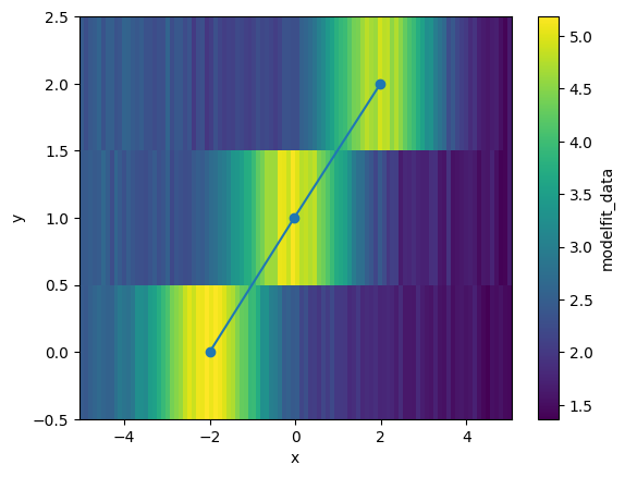
Let’s overlay the fitted peak positions on the data.
result_ds.modelfit_data.plot()
result_center = result_ds.sel(param="center")

plt.plot(result_center.modelfit_coefficients, result_center.y, "o-")
[<matplotlib.lines.Line2D at 0x702b46163f20>]
The same can be done with all parameter attributes that can be passed to lmfit.parameter.create_params() (e.g., vary, min, max, etc.). For example:
model = lmfit.models.GaussianModel() + lmfit.models.LinearModel()

params = {
    "center": {
        "value": xr.DataArray([-2, 0, 2], coords=[darr.y]),
        "min": -5.0,
        "max": xr.DataArray([0, 2, 5], coords=[darr.y]),
    },
    "slope": -0.1,
}

result_ds = darr.xlm.modelfit(coords="x", model=model, params=params)
result_ds
<xarray.Dataset> Size: 8kB
Dimensions:                (y: 3, param: 5, cov_i: 5, cov_j: 5, fit_stat: 9,
                            x: 100)
Coordinates:
  * y                      (y) int64 24B 0 1 2
  * x                      (x) float64 800B -5.0 -4.899 -4.798 ... 4.899 5.0
  * param                  (param) <U9 180B 'amplitude' 'center' ... 'intercept'
  * fit_stat               (fit_stat) <U8 288B 'nfev' 'nvarys' ... 'rsquared'
  * cov_i                  (cov_i) <U9 180B 'amplitude' 'center' ... 'intercept'
  * cov_j                  (cov_j) <U9 180B 'amplitude' 'center' ... 'intercept'
Data variables:
    modelfit_results       (y) object 24B <lmfit.model.ModelResult object at ...
    modelfit_coefficients  (y, param) float64 120B 7.324 -2.0 ... -0.1044 1.993
    modelfit_stderr        (y, param) float64 120B 0.1349 0.011 ... 0.01735
    modelfit_covariance    (y, cov_i, cov_j) float64 600B 0.01819 ... 0.000301
    modelfit_stats         (y, fit_stat) float64 216B 31.0 5.0 ... -450.2 0.9895
    modelfit_data          (y, x) float64 2kB 2.453 2.402 2.515 ... 1.404 1.64
modelfit_best_fit (y, x) float64 2kB 2.553 2.553 2.557 ... 1.526 1.504- y: 3
- param: 5
- cov_i: 5
- cov_j: 5
- fit_stat: 9
- x: 100
- y(y)int640 1 2
array([0, 1, 2])
- x(x)float64-5.0 -4.899 -4.798 ... 4.899 5.0
array([-5. , -4.89899 , -4.79798 , -4.69697 , -4.59596 , -4.494949, -4.393939, -4.292929, -4.191919, -4.090909, -3.989899, -3.888889, -3.787879, -3.686869, -3.585859, -3.484848, -3.383838, -3.282828, -3.181818, -3.080808, -2.979798, -2.878788, -2.777778, -2.676768, -2.575758, -2.474747, -2.373737, -2.272727, -2.171717, -2.070707, -1.969697, -1.868687, -1.767677, -1.666667, -1.565657, -1.464646, -1.363636, -1.262626, -1.161616, -1.060606, -0.959596, -0.858586, -0.757576, -0.656566, -0.555556, -0.454545, -0.353535, -0.252525, -0.151515, -0.050505, 0.050505, 0.151515, 0.252525, 0.353535, 0.454545, 0.555556, 0.656566, 0.757576, 0.858586, 0.959596, 1.060606, 1.161616, 1.262626, 1.363636, 1.464646, 1.565657, 1.666667, 1.767677, 1.868687, 1.969697, 2.070707, 2.171717, 2.272727, 2.373737, 2.474747, 2.575758, 2.676768, 2.777778, 2.878788, 2.979798, 3.080808, 3.181818, 3.282828, 3.383838, 3.484848, 3.585859, 3.686869, 3.787879, 3.888889, 3.989899, 4.090909, 4.191919, 4.292929, 4.393939, 4.494949, 4.59596 , 4.69697 , 4.79798 , 4.89899 , 5. ]) - param(param)<U9'amplitude' ... 'intercept'
array(['amplitude', 'center', 'sigma', 'slope', 'intercept'], dtype='<U9')
- fit_stat(fit_stat)<U8'nfev' 'nvarys' ... 'rsquared'
array(['nfev', 'nvarys', 'ndata', 'nfree', 'chisqr', 'redchi', 'aic', 'bic', 'rsquared'], dtype='<U8') - cov_i(cov_i)<U9'amplitude' ... 'intercept'
array(['amplitude', 'center', 'sigma', 'slope', 'intercept'], dtype='<U9')
- cov_j(cov_j)<U9'amplitude' ... 'intercept'
array(['amplitude', 'center', 'sigma', 'slope', 'intercept'], dtype='<U9')
- modelfit_results(y)object<lmfit.model.ModelResult object ...
array([<lmfit.model.ModelResult object at 0x702b461c66c0>, <lmfit.model.ModelResult object at 0x702b461b1c40>, <lmfit.model.ModelResult object at 0x702b461c70b0>], dtype=object) - modelfit_coefficients(y, param)float647.324 -2.0 0.9919 ... -0.1044 1.993
array([[ 7.32448001, -1.99999203, 0.99188961, -0.10520868, 1.99685627], [ 7.51733233, -0.02305536, 1.00038549, -0.09703458, 2.00966728], [ 7.59666334, 1.99366667, 0.99723597, -0.10435833, 1.99329924]]) - modelfit_stderr(y, param)float640.1349 0.011 ... 0.004993 0.01735
array([[0.13487916, 0.01099968, 0.0145665 , 0.00460002, 0.01594709], [0.10826445, 0.01195038, 0.0134014 , 0.00363877, 0.01476934], [0.14709905, 0.0115902 , 0.01537007, 0.00499338, 0.01734822]]) - modelfit_covariance(y, cov_i, cov_j)float640.01819 -0.0004108 ... 0.000301
array([[[ 1.81923884e-02, -4.10778631e-04, 1.61527298e-03, 4.48812633e-04, -1.78534512e-03], [-4.10778631e-04, 1.20992927e-04, -3.61601369e-05, -1.94837745e-05, 4.00282693e-05], [ 1.61527298e-03, -3.61601369e-05, 2.12182818e-04, 3.94797093e-05, -1.57975397e-04], [ 4.48812633e-04, -1.94837745e-05, 3.94797093e-05, 2.11601896e-05, -4.40240156e-05], [-1.78534512e-03, 4.00282693e-05, -1.57975397e-04, -4.40240156e-05, 2.54309769e-04]], [[ 1.17211909e-02, -3.23794933e-06, 1.03989216e-03, 3.42954185e-06, -1.16038832e-03], [-3.23794933e-06, 1.42811542e-04, -2.88200200e-07, -1.25021132e-05, 3.20525752e-07], [ 1.03989216e-03, -2.88200200e-07, 1.79597447e-04, 3.04294599e-07, -1.02947712e-04], [ 3.42954185e-06, -1.25021132e-05, 3.04294599e-07, 1.32406707e-05, -3.39519337e-07], [-1.16038832e-03, 3.20525752e-07, -1.02947712e-04, -3.39519337e-07, 2.18133476e-04]], [[ 2.16381297e-02, 4.77070169e-04, 1.86138075e-03, -5.32404156e-04, -2.12295084e-03], [ 4.77070169e-04, 1.34332621e-04, 4.06785606e-05, -2.24800417e-05, -4.64708628e-05], [ 1.86138075e-03, 4.06785606e-05, 2.36239011e-04, -4.53642459e-05, -1.81985967e-04], [-5.32404156e-04, -2.24800417e-05, -4.53642459e-05, 2.49338125e-05, 5.22093049e-05], [-2.12295084e-03, -4.64708628e-05, -1.81985967e-04, 5.22093049e-05, 3.00960582e-04]]]) - modelfit_stats(y, fit_stat)float6431.0 5.0 100.0 ... -450.2 0.9895
array([[ 3.10000000e+01, 5.00000000e+00, 1.00000000e+02, 9.50000000e+01, 7.51416422e-01, 7.90964655e-03, -4.79096548e+02, -4.66070697e+02, 9.94600761e-01], [ 3.10000000e+01, 5.00000000e+00, 1.00000000e+02, 9.50000000e+01, 9.80931827e-01, 1.03255982e-02, -4.52442250e+02, -4.39416399e+02, 9.91217434e-01], [ 3.10000000e+01, 5.00000000e+00, 1.00000000e+02, 9.50000000e+01, 8.80348758e-01, 9.26682904e-03, -4.63260732e+02, -4.50234881e+02, 9.89533284e-01]]) - modelfit_data(y, x)float642.453 2.402 2.515 ... 1.404 1.64
array([[2.45313385, 2.40235674, 2.51482263, 2.59074915, 2.6764208 , 2.59394952, 2.55499778, 2.56731807, 2.76560738, 2.90968187, 2.84053704, 2.76947573, 2.88970859, 3.25183004, 3.23198866, 3.17150326, 3.48156317, 3.52952886, 3.74747336, 3.93214775, 4.08299485, 4.38225482, 4.48844307, 4.59470196, 4.84031769, 5.0107361 , 4.87070097, 5.09207864, 5.07519126, 5.18226532, 5.06665073, 5.1631842 , 5.09310067, 4.9741113 , 4.78172815, 4.70632343, 4.47734082, 4.2766245 , 4.24965452, 3.9248589 , 3.95910191, 3.7214431 , 3.26250461, 3.30964501, 3.00234976, 2.95758539, 2.81323142, 2.47807647, 2.53524934, 2.42805834, 2.45768018, 2.16314796, 2.28587715, 2.04281712, 2.06893741, 1.97493843, 2.16724827, 2.04803446, 2.20774591, 2.005823 , 2.00617416, 1.98816284, 1.82771981, 1.8671122 , 1.99599647, 1.8089832 , 1.85582487, 1.82359101, 1.87574004, 1.76767498, 1.77844967, 1.80756538, 1.7833553 , 1.67633946, 1.84223817, 1.61266135, 1.61226509, 1.59400618, 1.80883879, 1.66597173, 1.59482299, 1.56822047, 1.7138329 , 1.55613362, 1.52430821, 1.70281395, 1.51164264, 1.58896847, 1.61043505, 1.55647661, 1.58549972, 1.71468544, 1.51901766, 1.43467535, 1.36683048, 1.51992743, 1.49507733, 1.54671111, 1.46367655, 1.45213615], ... [2.44598688, 2.27945239, 2.42172801, 2.46969848, 2.57847903, 2.34804814, 2.50606228, 2.50882285, 2.3492531 , 2.39033196, 2.57593497, 2.56093745, 2.46434024, 2.40188179, 2.47241732, 2.334418 , 2.32887606, 2.24224943, 2.31874259, 2.29988659, 2.57535533, 2.26861482, 2.40489271, 2.39977991, 2.23901312, 2.36454908, 2.01990284, 2.23709116, 2.30339681, 1.96804075, 2.08218813, 2.29416313, 2.15354763, 2.06045838, 2.12441002, 2.09962805, 2.21928705, 2.1862948 , 2.10839495, 2.06726183, 2.12816298, 2.26880543, 2.17763091, 2.21758283, 2.1550287 , 2.06379397, 2.15233711, 2.32770167, 2.32191728, 2.28119715, 2.28174929, 2.53935675, 2.59246129, 2.70310813, 2.83042558, 3.02980082, 3.18056376, 3.40698398, 3.57090932, 3.78336242, 3.90430899, 3.96129191, 4.15419323, 4.36316794, 4.42198394, 4.62833337, 4.78657269, 4.66322929, 4.61033938, 4.9210187 , 4.78721541, 4.80978954, 4.52997566, 4.73355509, 4.50666306, 4.27159498, 4.08309274, 3.9505857 , 3.73448627, 3.53049758, 3.25282672, 3.30031948, 2.98532803, 2.82062868, 2.65703864, 2.25870697, 2.40716854, 2.19504386, 2.08610797, 2.02225915, 1.83077418, 1.93668704, 1.71762378, 1.64110882, 1.59777002, 1.6594995 , 1.68388864, 1.52055751, 1.40397599, 1.63957606]]) - modelfit_best_fit(y, x)float642.553 2.553 2.557 ... 1.526 1.504
array([[2.55329433, 2.55341696, 2.55676688, 2.56410304, 2.57629343,
        2.59430927, 2.61921116, 2.65212582, 2.69421215, 2.7466161 ,
        2.81041428, 2.8865474 , 2.97574574, 3.07844962, 3.19472954,
        3.32421098, 3.46601014, 3.61868666, 3.78021955, 3.94801139,
        4.11892485, 4.28935335, 4.45532546, 4.61263995, 4.75702599,
        4.88432025, 4.99065099, 5.07261789, 5.12745602, 5.15317289,
        5.14864919, 5.11369604, 5.04906469, 4.95640801, 4.83819643,
        4.69759443, 4.53830606, 4.36440007, 4.18012617, 3.98973381,
        3.79730416, 3.60660414, 3.42096925, 3.24321924, 3.075608  ,
        2.91980684, 2.77691777, 2.64751218, 2.53168912, 2.42914678,
        2.33926125, 2.26116672, 2.19383246, 2.1361329 , 2.08690827,
        2.04501427, 2.00936047, 1.97893774, 1.95283567, 1.93025139,
        1.91049151, 1.89296855, 1.87719371, 1.86276721, 1.84936737,
        1.83673937, 1.82468442, 1.81304969, 1.80171935, 1.79060684,
        1.77964836, 1.76879751, 1.75802096, 1.74729513, 1.73660351,
        1.72593469, 1.7152809 , 1.70463691, 1.69399922, 1.68336556,
        1.67273442, 1.66210486, 1.65147627, 1.64084827, 1.63022063,
        1.6195932 , 1.60896589, 1.59833865, 1.58771146, 1.57708429,
        1.56645713, 1.55582999, 1.54520284, 1.5345757 , 1.52394856,
        1.51332142, 1.50269428, 1.49206714, 1.48144   , 1.47081286],
...
       [2.5150909 , 2.50454965, 2.49400841, 2.48346716, 2.47292592,
        2.46238467, 2.45184343, 2.44130219, 2.43076095, 2.42021971,
        2.40967849, 2.39913728, 2.3885961 , 2.37805498, 2.36751395,
        2.35697306, 2.34643244, 2.33589226, 2.32535278, 2.31481448,
        2.30427806, 2.29374464, 2.28321597, 2.27269471, 2.26218488,
        2.25169248, 2.2412264 , 2.23079956, 2.22043059, 2.21014595,
        2.1999828 , 2.18999263, 2.18024588, 2.17083755, 2.16189418,
        2.15358182, 2.14611543, 2.13976914, 2.13488731, 2.13189584,
        2.13131285, 2.13375804, 2.13995921, 2.1507548 , 2.1670906 ,
        2.1900093 , 2.22063102, 2.26012372, 2.30966249, 2.37037755,
        2.44329154, 2.5292477 , 2.62883175, 2.74229114, 2.86945683,
        3.00967299, 3.16174104, 3.32388401, 3.49373709, 3.66836867,
        3.84433491, 4.01776859, 4.18450033, 4.34020801, 4.48058733,
        4.60153457, 4.69933085, 4.77081636, 4.81354334, 4.82589738,
        4.80717868, 4.75763759, 4.67846188, 4.57171663, 4.44024106,
        4.28750941, 4.11746538, 3.93434122, 3.74247283, 3.54612219,
        3.34931691, 3.15571489, 2.96849976, 2.79030998, 2.62320209,
        2.46864623, 2.32754993, 2.20030525, 2.08685298, 1.98675791,
        1.89928902, 1.82349939, 1.75830144, 1.70253419, 1.65502055,
        1.61461332, 1.58023006, 1.55087715, 1.5256644 , 1.5038115 ]])
- yPandasIndex
PandasIndex(Index([0, 1, 2], dtype='int64', name='y'))
- xPandasIndex
PandasIndex(Index([ -5.0, -4.898989898989899, -4.797979797979798, -4.696969696969697, -4.595959595959596, -4.494949494949495, -4.393939393939394, -4.292929292929293, -4.191919191919192, -4.090909090909091, -3.9898989898989896, -3.888888888888889, -3.787878787878788, -3.686868686868687, -3.5858585858585856, -3.484848484848485, -3.383838383838384, -3.282828282828283, -3.1818181818181817, -3.080808080808081, -2.9797979797979797, -2.878787878787879, -2.7777777777777777, -2.676767676767677, -2.5757575757575757, -2.474747474747475, -2.3737373737373737, -2.272727272727273, -2.1717171717171717, -2.070707070707071, -1.9696969696969697, -1.868686868686869, -1.7676767676767677, -1.6666666666666665, -1.5656565656565657, -1.4646464646464645, -1.3636363636363638, -1.2626262626262625, -1.1616161616161618, -1.0606060606060606, -0.9595959595959593, -0.858585858585859, -0.7575757575757578, -0.6565656565656566, -0.5555555555555554, -0.45454545454545503, -0.3535353535353538, -0.2525252525252526, -0.15151515151515138, -0.050505050505050164, 0.050505050505050164, 0.15151515151515138, 0.2525252525252526, 0.3535353535353538, 0.45454545454545414, 0.5555555555555554, 0.6565656565656566, 0.7575757575757578, 0.8585858585858581, 0.9595959595959593, 1.0606060606060606, 1.1616161616161618, 1.262626262626262, 1.3636363636363633, 1.4646464646464645, 1.5656565656565657, 1.666666666666667, 1.7676767676767673, 1.8686868686868685, 1.9696969696969697, 2.070707070707071, 2.1717171717171713, 2.2727272727272725, 2.3737373737373737, 2.474747474747475, 2.5757575757575752, 2.6767676767676765, 2.7777777777777777, 2.878787878787879, 2.9797979797979792, 3.0808080808080813, 3.1818181818181817, 3.282828282828282, 3.383838383838384, 3.4848484848484844, 3.5858585858585865, 3.686868686868687, 3.787878787878787, 3.8888888888888893, 3.9898989898989896, 4.09090909090909, 4.191919191919192, 4.292929292929292, 4.3939393939393945, 4.494949494949495, 4.595959595959595, 4.696969696969697, 4.797979797979798, 4.8989898989899, 5.0], dtype='float64', name='x')) - paramPandasIndex
PandasIndex(Index(['amplitude', 'center', 'sigma', 'slope', 'intercept'], dtype='object', name='param'))
- fit_statPandasIndex
PandasIndex(Index(['nfev', 'nvarys', 'ndata', 'nfree', 'chisqr', 'redchi', 'aic', 'bic', 'rsquared'], dtype='object', name='fit_stat')) - cov_iPandasIndex
PandasIndex(Index(['amplitude', 'center', 'sigma', 'slope', 'intercept'], dtype='object', name='cov_i'))
- cov_jPandasIndex
PandasIndex(Index(['amplitude', 'center', 'sigma', 'slope', 'intercept'], dtype='object', name='cov_j'))
Parallelization#
The accessors are tightly integrated with xarray, so passing a dask array will
parallelize the fitting process. See Parallel Computing with Dask for background on how xarray and dask work together.
Assuming you have dask installed with a dask scheduler set up, you can fit large datasets in parallel with ease.
For example, recall the previous example where we created a DataArray with 3 Gaussian peaks, each with a different center, except this time we will create not just 3, but 300 peaks.
# Define coordinates
x = np.linspace(-5.0, 5.0, 100)
y = np.arange(300)

# Center of the peaks along y
center = np.linspace(-2.0, 2.0, 300)[:, np.newaxis]

# Gaussian peak on a linear background
z = -0.1 * x + 2 + 3 * np.exp(-((x - center) ** 2) / (2 * 1**2))

# Construct DataArray
darr = xr.DataArray(z, dims=["y", "x"], coords={"y": y, "x": x})
darr.plot()
<matplotlib.collections.QuadMesh at 0x702b4615e300>

Now, let’s try chunking the data and converting it to a dask array before fitting:
darr = darr.chunk({"y": 50})
darr
<xarray.DataArray (y: 300, x: 100)> Size: 240kB
dask.array<xarray-<this-array>, shape=(300, 100), dtype=float64, chunksize=(50, 100), chunktype=numpy.ndarray>
Coordinates:
  * y        (y) int64 2kB 0 1 2 3 4 5 6 7 8 ... 292 293 294 295 296 297 298 299
  * x        (x) float64 800B -5.0 -4.899 -4.798 -4.697 ... 4.798 4.899 5.0
- y: 300
- x: 100
- dask.array<chunksize=(50, 100), meta=np.ndarray>
Array Chunk Bytes 234.38 kiB 39.06 kiB Shape (300, 100) (50, 100) Dask graph 6 chunks in 1 graph layer Data type float64 numpy.ndarray - y(y)int640 1 2 3 4 5 ... 295 296 297 298 299
array([ 0, 1, 2, ..., 297, 298, 299], shape=(300,))
- x(x)float64-5.0 -4.899 -4.798 ... 4.899 5.0
array([-5.      , -4.89899 , -4.79798 , -4.69697 , -4.59596 , -4.494949,
       -4.393939, -4.292929, -4.191919, -4.090909, -3.989899, -3.888889,
       -3.787879, -3.686869, -3.585859, -3.484848, -3.383838, -3.282828,
       -3.181818, -3.080808, -2.979798, -2.878788, -2.777778, -2.676768,
       -2.575758, -2.474747, -2.373737, -2.272727, -2.171717, -2.070707,
       -1.969697, -1.868687, -1.767677, -1.666667, -1.565657, -1.464646,
       -1.363636, -1.262626, -1.161616, -1.060606, -0.959596, -0.858586,
       -0.757576, -0.656566, -0.555556, -0.454545, -0.353535, -0.252525,
       -0.151515, -0.050505,  0.050505,  0.151515,  0.252525,  0.353535,
        0.454545,  0.555556,  0.656566,  0.757576,  0.858586,  0.959596,
        1.060606,  1.161616,  1.262626,  1.363636,  1.464646,  1.565657,
        1.666667,  1.767677,  1.868687,  1.969697,  2.070707,  2.171717,
        2.272727,  2.373737,  2.474747,  2.575758,  2.676768,  2.777778,
        2.878788,  2.979798,  3.080808,  3.181818,  3.282828,  3.383838,
        3.484848,  3.585859,  3.686869,  3.787879,  3.888889,  3.989899,
        4.090909,  4.191919,  4.292929,  4.393939,  4.494949,  4.59596 ,
        4.69697 ,  4.79798 ,  4.89899 ,  5.      ])
- yPandasIndex
PandasIndex(Index([ 0, 1, 2, 3, 4, 5, 6, 7, 8, 9, ... 290, 291, 292, 293, 294, 295, 296, 297, 298, 299], dtype='int64', name='y', length=300)) - xPandasIndex
PandasIndex(Index([                 -5.0,    -4.898989898989899,    -4.797979797979798,
          -4.696969696969697,    -4.595959595959596,    -4.494949494949495,
          -4.393939393939394,    -4.292929292929293,    -4.191919191919192,
          -4.090909090909091,   -3.9898989898989896,    -3.888888888888889,
          -3.787878787878788,    -3.686868686868687,   -3.5858585858585856,
          -3.484848484848485,    -3.383838383838384,    -3.282828282828283,
         -3.1818181818181817,    -3.080808080808081,   -2.9797979797979797,
          -2.878787878787879,   -2.7777777777777777,    -2.676767676767677,
         -2.5757575757575757,    -2.474747474747475,   -2.3737373737373737,
          -2.272727272727273,   -2.1717171717171717,    -2.070707070707071,
         -1.9696969696969697,    -1.868686868686869,   -1.7676767676767677,
         -1.6666666666666665,   -1.5656565656565657,   -1.4646464646464645,
         -1.3636363636363638,   -1.2626262626262625,   -1.1616161616161618,
         -1.0606060606060606,   -0.9595959595959593,    -0.858585858585859,
         -0.7575757575757578,   -0.6565656565656566,   -0.5555555555555554,
        -0.45454545454545503,   -0.3535353535353538,   -0.2525252525252526,
        -0.15151515151515138, -0.050505050505050164,  0.050505050505050164,
         0.15151515151515138,    0.2525252525252526,    0.3535353535353538,
         0.45454545454545414,    0.5555555555555554,    0.6565656565656566,
          0.7575757575757578,    0.8585858585858581,    0.9595959595959593,
          1.0606060606060606,    1.1616161616161618,     1.262626262626262,
          1.3636363636363633,    1.4646464646464645,    1.5656565656565657,
           1.666666666666667,    1.7676767676767673,    1.8686868686868685,
          1.9696969696969697,     2.070707070707071,    2.1717171717171713,
          2.2727272727272725,    2.3737373737373737,     2.474747474747475,
          2.5757575757575752,    2.6767676767676765,    2.7777777777777777,
           2.878787878787879,    2.9797979797979792,    3.0808080808080813,
          3.1818181818181817,     3.282828282828282,     3.383838383838384,
          3.4848484848484844,    3.5858585858585865,     3.686868686868687,
           3.787878787878787,    3.8888888888888893,    3.9898989898989896,
            4.09090909090909,     4.191919191919192,     4.292929292929292,
          4.3939393939393945,     4.494949494949495,     4.595959595959595,
           4.696969696969697,     4.797979797979798,       4.8989898989899,
                         5.0],
      dtype='float64', name='x'))
When xarray.DataArray.xlm.modelfit() is called on a dask array, the fitting is not performed immediately. Instead, a dask graph is created that represents the computation to be performed:
model = lmfit.models.GaussianModel() + lmfit.models.LinearModel()

params = {
    "center": xr.DataArray(np.linspace(-2.0, 2.0, 300), coords=[darr.y]),
    "slope": -0.1,
}

result = darr.xlm.modelfit(coords="x", model=model, params=params)
result
<xarray.Dataset> Size: 592kB
Dimensions:                (y: 300, param: 5, cov_i: 5, cov_j: 5, fit_stat: 9,
                            x: 100)
Coordinates:
  * y                      (y) int64 2kB 0 1 2 3 4 5 ... 294 295 296 297 298 299
  * x                      (x) float64 800B -5.0 -4.899 -4.798 ... 4.899 5.0
  * param                  (param) <U9 180B 'amplitude' 'center' ... 'intercept'
  * fit_stat               (fit_stat) <U8 288B 'nfev' 'nvarys' ... 'rsquared'
  * cov_i                  (cov_i) <U9 180B 'amplitude' 'center' ... 'intercept'
  * cov_j                  (cov_j) <U9 180B 'amplitude' 'center' ... 'intercept'
Data variables:
    modelfit_results       (y) object 2kB dask.array<chunksize=(50,), meta=np.ndarray>
    modelfit_coefficients  (y, param) float64 12kB dask.array<chunksize=(50, 5), meta=np.ndarray>
    modelfit_stderr        (y, param) float64 12kB dask.array<chunksize=(50, 5), meta=np.ndarray>
    modelfit_covariance    (y, cov_i, cov_j) float64 60kB dask.array<chunksize=(50, 5, 5), meta=np.ndarray>
    modelfit_stats         (y, fit_stat) float64 22kB dask.array<chunksize=(50, 9), meta=np.ndarray>
    modelfit_data          (y, x) float64 240kB dask.array<chunksize=(50, 100), meta=np.ndarray>
modelfit_best_fit (y, x) float64 240kB dask.array<chunksize=(50, 100), meta=np.ndarray>- y: 300
- param: 5
- cov_i: 5
- cov_j: 5
- fit_stat: 9
- x: 100
- y(y)int640 1 2 3 4 5 ... 295 296 297 298 299
array([ 0, 1, 2, ..., 297, 298, 299], shape=(300,))
- x(x)float64-5.0 -4.899 -4.798 ... 4.899 5.0
array([-5. , -4.89899 , -4.79798 , -4.69697 , -4.59596 , -4.494949, -4.393939, -4.292929, -4.191919, -4.090909, -3.989899, -3.888889, -3.787879, -3.686869, -3.585859, -3.484848, -3.383838, -3.282828, -3.181818, -3.080808, -2.979798, -2.878788, -2.777778, -2.676768, -2.575758, -2.474747, -2.373737, -2.272727, -2.171717, -2.070707, -1.969697, -1.868687, -1.767677, -1.666667, -1.565657, -1.464646, -1.363636, -1.262626, -1.161616, -1.060606, -0.959596, -0.858586, -0.757576, -0.656566, -0.555556, -0.454545, -0.353535, -0.252525, -0.151515, -0.050505, 0.050505, 0.151515, 0.252525, 0.353535, 0.454545, 0.555556, 0.656566, 0.757576, 0.858586, 0.959596, 1.060606, 1.161616, 1.262626, 1.363636, 1.464646, 1.565657, 1.666667, 1.767677, 1.868687, 1.969697, 2.070707, 2.171717, 2.272727, 2.373737, 2.474747, 2.575758, 2.676768, 2.777778, 2.878788, 2.979798, 3.080808, 3.181818, 3.282828, 3.383838, 3.484848, 3.585859, 3.686869, 3.787879, 3.888889, 3.989899, 4.090909, 4.191919, 4.292929, 4.393939, 4.494949, 4.59596 , 4.69697 , 4.79798 , 4.89899 , 5. ]) - param(param)<U9'amplitude' ... 'intercept'
array(['amplitude', 'center', 'sigma', 'slope', 'intercept'], dtype='<U9')
- fit_stat(fit_stat)<U8'nfev' 'nvarys' ... 'rsquared'
array(['nfev', 'nvarys', 'ndata', 'nfree', 'chisqr', 'redchi', 'aic', 'bic', 'rsquared'], dtype='<U8') - cov_i(cov_i)<U9'amplitude' ... 'intercept'
array(['amplitude', 'center', 'sigma', 'slope', 'intercept'], dtype='<U9')
- cov_j(cov_j)<U9'amplitude' ... 'intercept'
array(['amplitude', 'center', 'sigma', 'slope', 'intercept'], dtype='<U9')
- modelfit_results(y)objectdask.array<chunksize=(50,), meta=np.ndarray>
Array Chunk Bytes 2.34 kiB 400 B Shape (300,) (50,) Dask graph 6 chunks in 7 graph layers Data type object numpy.ndarray - modelfit_coefficients(y, param)float64dask.array<chunksize=(50, 5), meta=np.ndarray>
Array Chunk Bytes 11.72 kiB 1.95 kiB Shape (300, 5) (50, 5) Dask graph 6 chunks in 7 graph layers Data type float64 numpy.ndarray - modelfit_stderr(y, param)float64dask.array<chunksize=(50, 5), meta=np.ndarray>
Array Chunk Bytes 11.72 kiB 1.95 kiB Shape (300, 5) (50, 5) Dask graph 6 chunks in 7 graph layers Data type float64 numpy.ndarray - modelfit_covariance(y, cov_i, cov_j)float64dask.array<chunksize=(50, 5, 5), meta=np.ndarray>
Array Chunk Bytes 58.59 kiB 9.77 kiB Shape (300, 5, 5) (50, 5, 5) Dask graph 6 chunks in 7 graph layers Data type float64 numpy.ndarray - modelfit_stats(y, fit_stat)float64dask.array<chunksize=(50, 9), meta=np.ndarray>
Array Chunk Bytes 21.09 kiB 3.52 kiB Shape (300, 9) (50, 9) Dask graph 6 chunks in 7 graph layers Data type float64 numpy.ndarray - modelfit_data(y, x)float64dask.array<chunksize=(50, 100), meta=np.ndarray>
Array Chunk Bytes 234.38 kiB 39.06 kiB Shape (300, 100) (50, 100) Dask graph 6 chunks in 7 graph layers Data type float64 numpy.ndarray - modelfit_best_fit(y, x)float64dask.array<chunksize=(50, 100), meta=np.ndarray>
Array Chunk Bytes 234.38 kiB 39.06 kiB Shape (300, 100) (50, 100) Dask graph 6 chunks in 7 graph layers Data type float64 numpy.ndarray
- yPandasIndex
PandasIndex(Index([ 0, 1, 2, 3, 4, 5, 6, 7, 8, 9, ... 290, 291, 292, 293, 294, 295, 296, 297, 298, 299], dtype='int64', name='y', length=300)) - xPandasIndex
PandasIndex(Index([ -5.0, -4.898989898989899, -4.797979797979798, -4.696969696969697, -4.595959595959596, -4.494949494949495, -4.393939393939394, -4.292929292929293, -4.191919191919192, -4.090909090909091, -3.9898989898989896, -3.888888888888889, -3.787878787878788, -3.686868686868687, -3.5858585858585856, -3.484848484848485, -3.383838383838384, -3.282828282828283, -3.1818181818181817, -3.080808080808081, -2.9797979797979797, -2.878787878787879, -2.7777777777777777, -2.676767676767677, -2.5757575757575757, -2.474747474747475, -2.3737373737373737, -2.272727272727273, -2.1717171717171717, -2.070707070707071, -1.9696969696969697, -1.868686868686869, -1.7676767676767677, -1.6666666666666665, -1.5656565656565657, -1.4646464646464645, -1.3636363636363638, -1.2626262626262625, -1.1616161616161618, -1.0606060606060606, -0.9595959595959593, -0.858585858585859, -0.7575757575757578, -0.6565656565656566, -0.5555555555555554, -0.45454545454545503, -0.3535353535353538, -0.2525252525252526, -0.15151515151515138, -0.050505050505050164, 0.050505050505050164, 0.15151515151515138, 0.2525252525252526, 0.3535353535353538, 0.45454545454545414, 0.5555555555555554, 0.6565656565656566, 0.7575757575757578, 0.8585858585858581, 0.9595959595959593, 1.0606060606060606, 1.1616161616161618, 1.262626262626262, 1.3636363636363633, 1.4646464646464645, 1.5656565656565657, 1.666666666666667, 1.7676767676767673, 1.8686868686868685, 1.9696969696969697, 2.070707070707071, 2.1717171717171713, 2.2727272727272725, 2.3737373737373737, 2.474747474747475, 2.5757575757575752, 2.6767676767676765, 2.7777777777777777, 2.878787878787879, 2.9797979797979792, 3.0808080808080813, 3.1818181818181817, 3.282828282828282, 3.383838383838384, 3.4848484848484844, 3.5858585858585865, 3.686868686868687, 3.787878787878787, 3.8888888888888893, 3.9898989898989896, 4.09090909090909, 4.191919191919192, 4.292929292929292, 4.3939393939393945, 4.494949494949495, 4.595959595959595, 4.696969696969697, 4.797979797979798, 4.8989898989899, 5.0], dtype='float64', name='x')) - paramPandasIndex
PandasIndex(Index(['amplitude', 'center', 'sigma', 'slope', 'intercept'], dtype='object', name='param'))
- fit_statPandasIndex
PandasIndex(Index(['nfev', 'nvarys', 'ndata', 'nfree', 'chisqr', 'redchi', 'aic', 'bic', 'rsquared'], dtype='object', name='fit_stat')) - cov_iPandasIndex
PandasIndex(Index(['amplitude', 'center', 'sigma', 'slope', 'intercept'], dtype='object', name='cov_i'))
- cov_jPandasIndex
PandasIndex(Index(['amplitude', 'center', 'sigma', 'slope', 'intercept'], dtype='object', name='cov_j'))
You can call .compute() on the entire Dataset, or on individual variables to perform the fitting in parallel.
result.compute()
<xarray.Dataset> Size: 592kB
Dimensions:                (y: 300, param: 5, cov_i: 5, cov_j: 5, fit_stat: 9,
                            x: 100)
Coordinates:
  * y                      (y) int64 2kB 0 1 2 3 4 5 ... 294 295 296 297 298 299
  * x                      (x) float64 800B -5.0 -4.899 -4.798 ... 4.899 5.0
  * param                  (param) <U9 180B 'amplitude' 'center' ... 'intercept'
  * fit_stat               (fit_stat) <U8 288B 'nfev' 'nvarys' ... 'rsquared'
  * cov_i                  (cov_i) <U9 180B 'amplitude' 'center' ... 'intercept'
  * cov_j                  (cov_j) <U9 180B 'amplitude' 'center' ... 'intercept'
Data variables:
    modelfit_results       (y) object 2kB <lmfit.model.ModelResult object at ...
    modelfit_coefficients  (y, param) float64 12kB 7.52 -2.0 1.0 ... -0.1 2.0
    modelfit_stderr        (y, param) float64 12kB 6.986e-15 ... 1.121e-15
    modelfit_covariance    (y, cov_i, cov_j) float64 60kB 4.881e-29 ... 1.256...
    modelfit_stats         (y, fit_stat) float64 22kB 13.0 5.0 ... 1.0
    modelfit_data          (y, x) float64 240kB 2.533 2.535 2.54 ... 1.555 1.533
modelfit_best_fit (y, x) float64 240kB 2.533 2.535 2.54 ... 1.555 1.533- y: 300
- param: 5
- cov_i: 5
- cov_j: 5
- fit_stat: 9
- x: 100
- y(y)int640 1 2 3 4 5 ... 295 296 297 298 299
array([ 0, 1, 2, ..., 297, 298, 299], shape=(300,))
- x(x)float64-5.0 -4.899 -4.798 ... 4.899 5.0
array([-5. , -4.89899 , -4.79798 , -4.69697 , -4.59596 , -4.494949, -4.393939, -4.292929, -4.191919, -4.090909, -3.989899, -3.888889, -3.787879, -3.686869, -3.585859, -3.484848, -3.383838, -3.282828, -3.181818, -3.080808, -2.979798, -2.878788, -2.777778, -2.676768, -2.575758, -2.474747, -2.373737, -2.272727, -2.171717, -2.070707, -1.969697, -1.868687, -1.767677, -1.666667, -1.565657, -1.464646, -1.363636, -1.262626, -1.161616, -1.060606, -0.959596, -0.858586, -0.757576, -0.656566, -0.555556, -0.454545, -0.353535, -0.252525, -0.151515, -0.050505, 0.050505, 0.151515, 0.252525, 0.353535, 0.454545, 0.555556, 0.656566, 0.757576, 0.858586, 0.959596, 1.060606, 1.161616, 1.262626, 1.363636, 1.464646, 1.565657, 1.666667, 1.767677, 1.868687, 1.969697, 2.070707, 2.171717, 2.272727, 2.373737, 2.474747, 2.575758, 2.676768, 2.777778, 2.878788, 2.979798, 3.080808, 3.181818, 3.282828, 3.383838, 3.484848, 3.585859, 3.686869, 3.787879, 3.888889, 3.989899, 4.090909, 4.191919, 4.292929, 4.393939, 4.494949, 4.59596 , 4.69697 , 4.79798 , 4.89899 , 5. ]) - param(param)<U9'amplitude' ... 'intercept'
array(['amplitude', 'center', 'sigma', 'slope', 'intercept'], dtype='<U9')
- fit_stat(fit_stat)<U8'nfev' 'nvarys' ... 'rsquared'
array(['nfev', 'nvarys', 'ndata', 'nfree', 'chisqr', 'redchi', 'aic', 'bic', 'rsquared'], dtype='<U8') - cov_i(cov_i)<U9'amplitude' ... 'intercept'
array(['amplitude', 'center', 'sigma', 'slope', 'intercept'], dtype='<U9')
- cov_j(cov_j)<U9'amplitude' ... 'intercept'
array(['amplitude', 'center', 'sigma', 'slope', 'intercept'], dtype='<U9')
- modelfit_results(y)object<lmfit.model.ModelResult object ...
array([<lmfit.model.ModelResult object at 0x702b4188ddf0>, <lmfit.model.ModelResult object at 0x702b4188fa40>, <lmfit.model.ModelResult object at 0x702b4188e600>, <lmfit.model.ModelResult object at 0x702b4188fe90>, <lmfit.model.ModelResult object at 0x702b4188f500>, <lmfit.model.ModelResult object at 0x702b417ed2b0>, <lmfit.model.ModelResult object at 0x702b4188c5c0>, <lmfit.model.ModelResult object at 0x702b416ea3c0>, <lmfit.model.ModelResult object at 0x702b4188f140>, <lmfit.model.ModelResult object at 0x702b416e9c40>, <lmfit.model.ModelResult object at 0x702b416ea2d0>, <lmfit.model.ModelResult object at 0x702b41848d40>, <lmfit.model.ModelResult object at 0x702b4172e540>, <lmfit.model.ModelResult object at 0x702b4194ee70>, <lmfit.model.ModelResult object at 0x702b4188f3b0>, <lmfit.model.ModelResult object at 0x702b4172e780>, <lmfit.model.ModelResult object at 0x702b416eaa80>, <lmfit.model.ModelResult object at 0x702b4172fd40>, <lmfit.model.ModelResult object at 0x702b416e9dc0>, <lmfit.model.ModelResult object at 0x702b417ee210>, ... <lmfit.model.ModelResult object at 0x702b43407740>, <lmfit.model.ModelResult object at 0x702b43593e00>, <lmfit.model.ModelResult object at 0x702b43406b40>, <lmfit.model.ModelResult object at 0x702b434021e0>, <lmfit.model.ModelResult object at 0x702b43405d60>, <lmfit.model.ModelResult object at 0x702b434d4ef0>, <lmfit.model.ModelResult object at 0x702b43593d70>, <lmfit.model.ModelResult object at 0x702b43416ff0>, <lmfit.model.ModelResult object at 0x702b43578c80>, <lmfit.model.ModelResult object at 0x702b43400bf0>, <lmfit.model.ModelResult object at 0x702b43415040>, <lmfit.model.ModelResult object at 0x702b43414e00>, <lmfit.model.ModelResult object at 0x702b432f2030>, <lmfit.model.ModelResult object at 0x702b43416fc0>, <lmfit.model.ModelResult object at 0x702b43415f40>, <lmfit.model.ModelResult object at 0x702b432f0e00>, <lmfit.model.ModelResult object at 0x702b432f3770>, <lmfit.model.ModelResult object at 0x702b432f12e0>, <lmfit.model.ModelResult object at 0x702b432f1a00>, <lmfit.model.ModelResult object at 0x702b432f3980>], dtype=object) - modelfit_coefficients(y, param)float647.52 -2.0 1.0 -0.1 ... 1.0 -0.1 2.0
array([[ 7.51988482, -2. , 1. , -0.1 , 2. ], [ 7.51988482, -1.98662207, 1. , -0.1 , 2. ], [ 7.51988482, -1.97324415, 1. , -0.1 , 2. ], ..., [ 7.51988482, 1.97324415, 1. , -0.1 , 2. ], [ 7.51988482, 1.98662207, 1. , -0.1 , 2. ], [ 7.51988482, 2. , 1. , -0.1 , 2. ]], shape=(300, 5)) - modelfit_stderr(y, param)float646.986e-15 5.546e-16 ... 1.121e-15
array([[6.98625366e-15, 5.54615850e-16, 7.37505007e-16, 2.36623994e-16, 8.21655993e-16], [1.75024863e-14, 1.39662679e-15, 1.85198954e-15, 5.92663102e-16, 2.06269958e-15], [4.35157344e-15, 3.49012109e-16, 4.61524685e-16, 1.47316328e-16, 5.13887691e-16], ..., [8.57720391e-15, 6.87923132e-16, 9.09688879e-16, 2.90369035e-16, 1.01290248e-15], [1.95690355e-15, 1.56152896e-16, 2.07065008e-16, 6.62639872e-17, 2.30624613e-16], [9.52814127e-15, 7.56408001e-16, 1.00583628e-15, 3.22717576e-16, 1.12060838e-15]], shape=(300, 5)) - modelfit_covariance(y, cov_i, cov_j)float644.881e-29 -1.098e-30 ... 1.256e-30
array([[[ 4.88077403e-29, -1.09775754e-30, 4.25000363e-30, 1.20426396e-30, -4.78675488e-30], [-1.09775754e-30, 3.07598741e-31, -9.47354635e-32, -5.13611581e-32, 1.06870164e-31], [ 4.25000363e-30, -9.47354635e-32, 5.43913635e-31, 1.03841903e-31, -4.15318126e-31], [ 1.20426396e-30, -5.13611581e-32, 1.03841903e-31, 5.59909148e-32, -1.18046900e-31], [-4.78675488e-30, 1.06870164e-31, -4.15318126e-31, -1.18046900e-31, 6.75118572e-31]], [[ 3.06337028e-28, -6.85842160e-30, 2.66927915e-29, 7.51462017e-30, -3.00540730e-29], [-6.85842160e-30, 1.95056639e-30, -5.92361915e-31, -3.22564056e-31, 6.68041271e-31], [ 2.66927915e-29, -5.92361915e-31, 3.42986525e-30, 6.48536470e-31, -2.60961667e-30], [ 7.51462017e-30, -3.22564056e-31, 6.48536470e-31, 3.51249552e-31, -7.36877307e-31], [-3.00540730e-29, 6.68041271e-31, -2.60961667e-30, ... -9.39390976e-32, -3.75701290e-31], [ 8.57360614e-32, 2.43837269e-32, 7.40453972e-33, -4.03232307e-33, -8.35108000e-33], [ 3.33680730e-31, 7.40453972e-33, 4.28759177e-32, -8.10717340e-33, -3.26222460e-32], [-9.39390976e-32, -4.03232307e-33, -8.10717340e-33, 4.39091599e-33, 9.21158857e-33], [-3.75701290e-31, -8.35108000e-33, -3.26222460e-32, 9.21158857e-33, 5.31877119e-32]], [[ 9.07854760e-29, 2.04189827e-30, 7.90523403e-30, -2.24000694e-30, -8.90366605e-30], [ 2.04189827e-30, 5.72153063e-31, 1.76202495e-31, -9.55349942e-32, -1.98785247e-31], [ 7.90523403e-30, 1.76202495e-31, 1.01170663e-30, -1.93150580e-31, -7.72513939e-31], [-2.24000694e-30, -9.55349942e-32, -1.93150580e-31, 1.04146634e-31, 2.19574681e-31], [-8.90366605e-30, -1.98785247e-31, -7.72513939e-31, 2.19574681e-31, 1.25576314e-30]]], shape=(300, 5, 5)) - modelfit_stats(y, fit_stat)float6413.0 5.0 100.0 ... -6.525e+03 1.0
array([[ 1.30000000e+01, 5.00000000e+00, 1.00000000e+02, ..., -6.60052615e+03, -6.58750029e+03, 1.00000000e+00], [ 1.30000000e+01, 5.00000000e+00, 1.00000000e+02, ..., -6.41566308e+03, -6.40263723e+03, 1.00000000e+00], [ 1.30000000e+01, 5.00000000e+00, 1.00000000e+02, ..., -6.69285164e+03, -6.67982579e+03, 1.00000000e+00], ..., [ 1.30000000e+01, 5.00000000e+00, 1.00000000e+02, ..., -6.55713755e+03, -6.54411170e+03, 1.00000000e+00], [ 1.30000000e+01, 5.00000000e+00, 1.00000000e+02, ..., -6.85385899e+03, -6.84083314e+03, 1.00000000e+00], [ 1.30000000e+01, 5.00000000e+00, 1.00000000e+02, ..., -6.53846510e+03, -6.52543925e+03, 1.00000000e+00]], shape=(300, 9)) - modelfit_data(y, x)float642.533 2.535 2.54 ... 1.555 1.533
array([[2.53332699, 2.53479264, 2.53965879, ..., 1.52020202, 1.51010101, 1.5 ], [2.53201307, 2.53308102, 2.53745439, ..., 1.52020202, 1.51010101, 1.5 ], [2.53074545, 2.53142722, 2.53532123, ..., 1.52020202, 1.51010101, 1.5 ], ..., [2.5 , 2.48989899, 2.47979798, ..., 1.57572527, 1.55162924, 1.53074545], [2.5 , 2.48989899, 2.47979798, ..., 1.57785843, 1.55328304, 1.53201307], [2.5 , 2.48989899, 2.47979798, ..., 1.58006283, 1.55499466, 1.53332699]], shape=(300, 100)) - modelfit_best_fit(y, x)float642.533 2.535 2.54 ... 1.555 1.533
array([[2.53332699, 2.53479264, 2.53965879, ..., 1.52020202, 1.51010101,
        1.5       ],
       [2.53201307, 2.53308102, 2.53745439, ..., 1.52020202, 1.51010101,
        1.5       ],
       [2.53074545, 2.53142722, 2.53532123, ..., 1.52020202, 1.51010101,
        1.5       ],
       ...,
       [2.5       , 2.48989899, 2.47979798, ..., 1.57572527, 1.55162924,
        1.53074545],
       [2.5       , 2.48989899, 2.47979798, ..., 1.57785843, 1.55328304,
        1.53201307],
       [2.5       , 2.48989899, 2.47979798, ..., 1.58006283, 1.55499466,
        1.53332699]], shape=(300, 100))
- yPandasIndex
PandasIndex(Index([ 0, 1, 2, 3, 4, 5, 6, 7, 8, 9, ... 290, 291, 292, 293, 294, 295, 296, 297, 298, 299], dtype='int64', name='y', length=300)) - xPandasIndex
PandasIndex(Index([ -5.0, -4.898989898989899, -4.797979797979798, -4.696969696969697, -4.595959595959596, -4.494949494949495, -4.393939393939394, -4.292929292929293, -4.191919191919192, -4.090909090909091, -3.9898989898989896, -3.888888888888889, -3.787878787878788, -3.686868686868687, -3.5858585858585856, -3.484848484848485, -3.383838383838384, -3.282828282828283, -3.1818181818181817, -3.080808080808081, -2.9797979797979797, -2.878787878787879, -2.7777777777777777, -2.676767676767677, -2.5757575757575757, -2.474747474747475, -2.3737373737373737, -2.272727272727273, -2.1717171717171717, -2.070707070707071, -1.9696969696969697, -1.868686868686869, -1.7676767676767677, -1.6666666666666665, -1.5656565656565657, -1.4646464646464645, -1.3636363636363638, -1.2626262626262625, -1.1616161616161618, -1.0606060606060606, -0.9595959595959593, -0.858585858585859, -0.7575757575757578, -0.6565656565656566, -0.5555555555555554, -0.45454545454545503, -0.3535353535353538, -0.2525252525252526, -0.15151515151515138, -0.050505050505050164, 0.050505050505050164, 0.15151515151515138, 0.2525252525252526, 0.3535353535353538, 0.45454545454545414, 0.5555555555555554, 0.6565656565656566, 0.7575757575757578, 0.8585858585858581, 0.9595959595959593, 1.0606060606060606, 1.1616161616161618, 1.262626262626262, 1.3636363636363633, 1.4646464646464645, 1.5656565656565657, 1.666666666666667, 1.7676767676767673, 1.8686868686868685, 1.9696969696969697, 2.070707070707071, 2.1717171717171713, 2.2727272727272725, 2.3737373737373737, 2.474747474747475, 2.5757575757575752, 2.6767676767676765, 2.7777777777777777, 2.878787878787879, 2.9797979797979792, 3.0808080808080813, 3.1818181818181817, 3.282828282828282, 3.383838383838384, 3.4848484848484844, 3.5858585858585865, 3.686868686868687, 3.787878787878787, 3.8888888888888893, 3.9898989898989896, 4.09090909090909, 4.191919191919192, 4.292929292929292, 4.3939393939393945, 4.494949494949495, 4.595959595959595, 4.696969696969697, 4.797979797979798, 4.8989898989899, 5.0], dtype='float64', name='x')) - paramPandasIndex
PandasIndex(Index(['amplitude', 'center', 'sigma', 'slope', 'intercept'], dtype='object', name='param'))
- fit_statPandasIndex
PandasIndex(Index(['nfev', 'nvarys', 'ndata', 'nfree', 'chisqr', 'redchi', 'aic', 'bic', 'rsquared'], dtype='object', name='fit_stat')) - cov_iPandasIndex
PandasIndex(Index(['amplitude', 'center', 'sigma', 'slope', 'intercept'], dtype='object', name='cov_i'))
- cov_jPandasIndex
PandasIndex(Index(['amplitude', 'center', 'sigma', 'slope', 'intercept'], dtype='object', name='cov_j'))